Temperature Control in Heat Exchanger

Open Live Script

This example shows how to design feedback and feedforward compensators to regulate the temperature of a chemical reactor through a heat exchanger.

Heat Exchanger Process

A chemical reactor called a stirring tank is depicted below. The top inlet delivers liquid to be mixed in the tank. The tank liquid must be maintained at a constant temperature by varying the amount of steam supplied to the heat exchanger (bottom pipe) via its control valve. Variations in the temperature of the inlet flow are the main source of disturbances in this process.

Using Measured Data to Model Heat Exchanger Dynamics

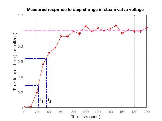
To derive a first-order-plus-deadtime model of the heat exchanger characteristics, inject a step disturbance in valve voltage V and record the effect on the tank temperature T over time. Load and plot the experimental data.

load("step_data.mat","tData","yData")

plot(tData,yData,"r*-")
xlim([0 200])
ylim([0 1.2])
ylabel("Tank temperature (normalized)")
xlabel ("Time (seconds)")
grid on;
title("Measured Step Response");

hold on
t1 = 23;
t2 = 36;
plot([t1 t1],[0 0.283],"b--",LineWidth=2)
plot([0 t1],[0.283 0.283],"b--",LineWidth=2)
annotation("textbox",[0.22 0.26 0.1 0.1], ...
    String="t1",Color="b",EdgeColor="none")
plot([t2 t2],[0 0.632],"b--",LineWidth=2)
plot([0 t2],[0.632 0.632],"b--",LineWidth=2)
annotation("textbox",[0.28 0.48 0.1 0.1], ...
    String="t2",Color="b",EdgeColor="none")

Figure contains an axes object. The axes object with title Measured Step Response, xlabel Time (seconds), ylabel Tank temperature (normalized) contains 5 objects of type line.

The values t1 and t2 are the times where the response attains 28.3% and 63.2% of its final value. You can use these values to estimate the time constant tau and dead time theta for the heat exchanger.

tau = 3/2 * ( t2 - t1 )

tau = 
19.5000

theta = t2 - tau

theta = 
16.5000

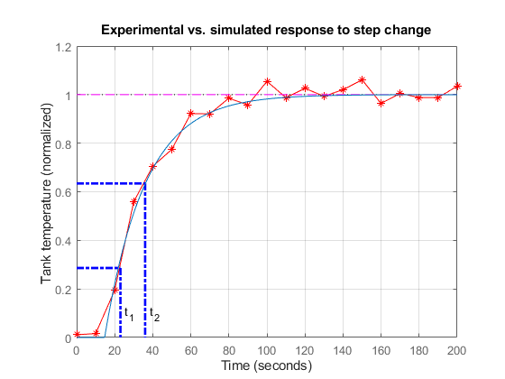
Verify these calculations by comparing the first-order-plus-dead-time response with the measured response.

s = tf("s");
Gp = exp(-theta*s)/(1+tau*s);

Plot the step response of Gp on the same axes as the the experimental data.

sp = stepplot(Gp,0:1:200);
xlim([0 200])
ylim([0 1.2])
ylabel("Tank temperature (normalized)")

ans = 
  AxesLabel with properties:

         String: "Tank temperature (normalized)"
       FontSize: 11
     FontWeight: "normal"
      FontAngle: "normal"
          Color: [0.1500 0.1500 0.1500]
    Interpreter: "tex"
        Visible: on

title("Experimental and Simulated Step Response")
grid on

MATLAB figure

The model response and the experimental data are in good agreement. A similar bump test experiment could be conducted to estimate the first-order response to a step disturbance in inflow temperature. Equipped with models for the heat exchanger and inflow disturbance, you are ready to design the control algorithm.

Feedback Control

The following figure shows a block diagram of the open-loop process.

The transfer function

$G_{p} (s) = \frac{e^{- 14.7 s}}{21.3 s + 1}$

models how a change in the voltage V driving the steam valve opening affects the tank temperature T, while the transfer function

$G_{d} (s) = \frac{e^{- 35 s}}{25 s + 1}$

models how a change d in inflow temperature affects T. To regulate the tank temperature T around a given setpoint Tsp, you can use the following feedback architecture to control the valve opening (voltage V).

In this configuration, the proportional-integral (PI) controller

$C (s) = K_{c} (1 + \frac{1}{τ_{c} s})$

calculates the voltage V based on the gap Tsp-T between the desired and measured temperatures. You can use the ITAE formulas to pick adequate values for the controller parameters.

$K_{c} = 0.859 (θ / τ)^{- 0.977}, τ_{c} = (θ / τ)^{0.680} τ / 0.674$

Kc = 0.859 * (theta / tau)^(-0.977)

Kc = 
1.0113

tauc = ( tau / 0.674 ) * ( theta / tau )^0.680

tauc = 
25.8250

C = Kc * (1 + 1/(tauc*s));

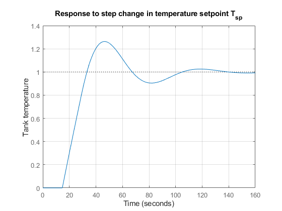
To see how well the ITAE controller performs, close the feedback loop and simulate the response to a setpoint change.

figure
Tfb = feedback(ss(Gp*C),1);
stepplot(Tfb,0:1:200)
hold on
plot(tData,yData,"r*-")
title("Response to Step Change in Temperature Setpoint")
ylabel("Tank temperature (normalized)")

ans = 
  AxesLabel with properties:

         String: "Tank temperature (normalized)"
       FontSize: 11
     FontWeight: "normal"
      FontAngle: "normal"
          Color: [0.1500 0.1500 0.1500]
    Interpreter: "tex"
        Visible: on

grid on

MATLAB figure

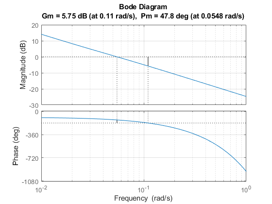
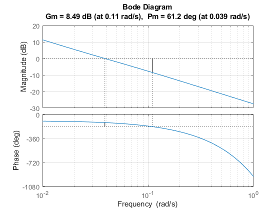
The response is fairly fast with some overshoot. Looking at the stability margins confirms that the gain margin is weak.

figure
margin(Gp*C)
grid on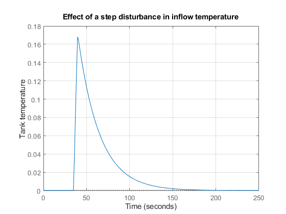

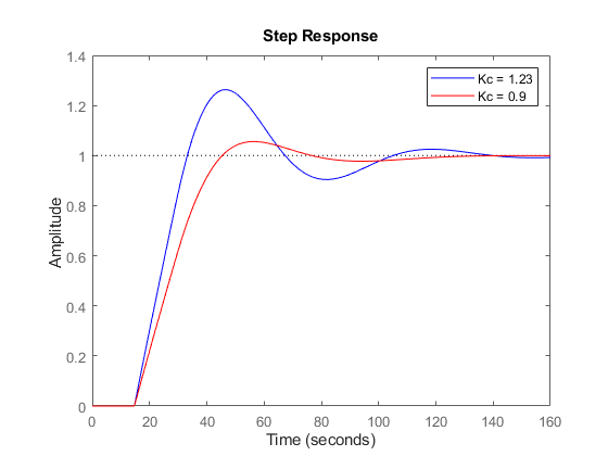
MATLAB figure

Reducing the proportional gain Kc strengthens stability at the expense of performance.

C1 = 0.9 * (1 + 1/(tauc*s));  % reduce Kc from 1.23 to 0.9
margin(Gp*C1)
grid on

MATLAB figure

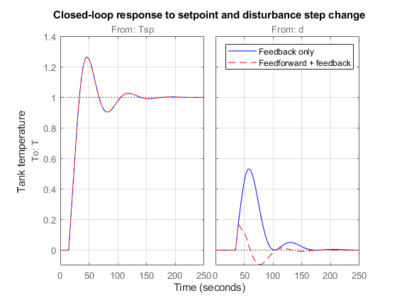
figure
stepplot(Tfb,"r",feedback(ss(Gp*C1),1),"b",0:1:200)
title("Response to Step Change in Temperature Setpoint")
ylabel("Tank temperature (normalized)")

ans = 
  AxesLabel with properties:

         String: "Tank temperature (normalized)"
       FontSize: 11
     FontWeight: "normal"
      FontAngle: "normal"
          Color: [0.1500 0.1500 0.1500]
    Interpreter: "tex"
        Visible: on

legend("Kc = 1.23","Kc = 0.9");
grid on

MATLAB figure

Feedforward Control

Recall that changes in inflow temperature are the main source of temperature fluctuations in the tank. To reject such disturbances, an alternative to feedback control is the feedforward architecture shown below:

In this configuration, the feedforward controller F uses measurements of the inflow temperature to adjust the steam valve opening (voltage V). Feedforward control thus anticipates and preempts the effect of inflow temperature changes.

Straightforward calculation shows that the overall transfer from temperature disturbance d to tank temperature T is

$T = (G_{p} F + G_{d}) d$

Perfect disturbance rejection requires

$G_{p} F + G_{d} = 0 \to F = - \frac{G_{d}}{G_{p}} = - \frac{21.3 s + 1}{25 s + 1} e^{- 20.3 s}$

In reality, modeling inaccuracies prevent exact disturbance rejection, but feedforward control will help minimize temperature fluctuations due to inflow disturbances. To get a better sense of how the feedforward scheme would perform, increase the ideal feedforward delay by 5 seconds and simulate the response to a step change in inflow temperature:

Gd = exp(-35*s)/(25*s+1);
F = -(21.3*s+1)/(25*s+1) * exp(-25*s);
Tff = Gp * ss(F) + Gd;   % d->T transfer with feedforward control

figure
stepplot(Tff)
title("Effect of Step Disturbance in Inflow Temperature")
ylabel("Tank temperature (normalized)")

ans = 
  AxesLabel with properties:

         String: "Tank temperature (normalized)"
       FontSize: 11
     FontWeight: "normal"
      FontAngle: "normal"
          Color: [0.1500 0.1500 0.1500]
    Interpreter: "tex"
        Visible: on

grid on

MATLAB figure

Combined Feedforward-Feedback Control

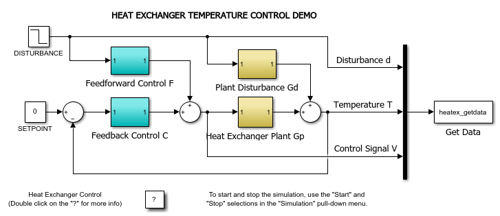
Feedback control is good for setpoint tracking in general, while feedforward control can help with rejection of measured disturbances. Next, look at the benefits of combining both schemes. The corresponding control architecture is shown in the following figure.

Use connect to build the corresponding closed-loop model from Tsp,d to T. First name the input and output channels of each block, then use connect to wire the diagram.

Gd.u = "d";
Gd.y = "Td";
Gp.u = "V";
Gp.y = "Tp";
F.u = "d";
F.y = "Vf";
C.u = "e";
C.y = "Vc";
Sum1 = sumblk("e = Tsp - T");
Sum2 = sumblk("V = Vf + Vc");
Sum3 = sumblk("T = Tp + Td");
Tffb = connect(Gp,Gd,C,F,Sum1,Sum2,Sum3,{"Tsp","d"},"T");

To compare the closed-loop responses with and without feedforward control, calculate the corresponding closed-loop transfer function for the feedback-only configuration.

C.u = "e";
C.y = "V";
Tfb = connect(Gp,Gd,C,Sum1,Sum3,{"Tsp","d"},"T");

Compare the two designs.

stepplot(Tfb,"b",Tffb,"r--");
title("Closed-loop Step Response to Setpoint and Disturbance Change");
ylabel("Tank temperature (normalized)")

ans = 
  AxesLabel with properties:

         String: "Tank temperature (normalized)"
       FontSize: 11
     FontWeight: "normal"
      FontAngle: "normal"
          Color: [0.1500 0.1500 0.1500]
    Interpreter: "tex"
        Visible: on

legend("Feedback only","Feedforward + feedback");
grid on

MATLAB figure

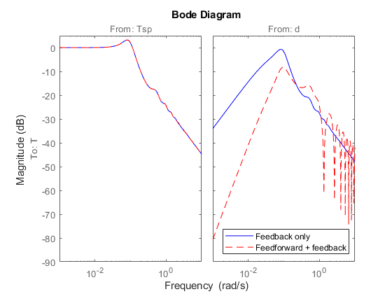
The two designs have identical performance for setpoint tracking, but the addition of feedforward control improves disturbance rejection. This result is also visible on the closed-loop Bode plot.

figure
bodemag(Tfb,"b",Tffb,"r--",{1e-3,1e1})
legend("Feedback only","Feedforward + feedback",Location="SouthEast");

MATLAB figure

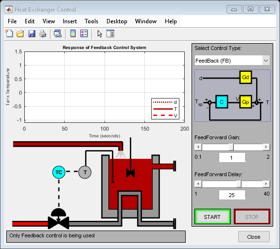
Interactive Simulation

You can use the HeatExchanger app to interactively explore cotnrol strategies for the heat exchanger system. The app was developed using App Designer and simulates the heat exchnager using the heatex_sim Simulink® model.

Using this app, you can simulate the heat exchanger using open-loop, feedforward, feedback, and combined feedforward-feedback control. You can also adjust the gain and delay parameters for the feedforward controller.

To run the app, use the following command.

HeatExchanger