Floating-Point to Fixed-Point Conversion of IIR Filters
This example shows how to use the Fixed-Point Converter App to convert an IIR filter from a floating-point to a fixed-point implementation. Second-order sections (also referred as biquadratic) structures work better when using fixed-point arithmetic than structures that implement the transfer function directly. We will show that the surest path to a successful "float-to-fixed" conversion consists of the following steps:
Select a Second-Order Sections (SOS) structure, i.e.
dsp.BiquadFilterPerform dynamic range analysis for each node of the filter, i.e. use a test bench approach with simulation minimum and simulation maximum instrumentation
Compare alternative biquadratic scaling implementations and view quantization effects due to different choices using '
fvtool' and spectrumAnalyzerfor analysis and verification.
Introduction
An efficient way to implement an IIR filter is using a Second Order Section (SOS) Biquad filter structure. Suppose for example that we need to remove an interfering high frequency tone signal from a system. One way to achieve this is to use a lowpass filter design.
Design a Lowpass Elliptic Filter
Use a minimum-order lowpass Elliptic Direct-Form I design for the purpose of this example. The design specifications of the filter are:
Passband frequency edge:
Stopband frequency edge:
Passband ripple:
Stopband attenuation:
Visualize the cumulative filter response of all the second-order sections using the Filter Visualization Tool.
biquad = design(fdesign.lowpass('Fp,Fst,Ap,Ast',0.4,0.45,0.5,80), ...
    'ellip',FilterStructure='df1sos', SystemObject=true, UseLegacyBiquadFilter=true);
fvt = fvtool(biquad, Legend='on');
fvt.SosviewSettings.View = 'Cumulative';
![{"String":"Figure Figure 1: Magnitude Response (dB) contains an axes object. The axes object with title Magnitude Response (dB) contains 5 objects of type line. These objects represent Filter #1: Section #1, Filter #1: Sections #1-2, Filter #1: Sections #1-3, Filter #1: Sections #1-4, Filter #1: Sections #1-5.","Tex":"Magnitude Response (dB)","LaTex":[]}](../../examples/dsp/win64/FloatingPointToFixedPointConversionOfIIRFiltersExample_01.png)
Obtain Filter Coefficients (SOS, B, A) for Float vs. Fixed Comparison
Note that the SOS filter coefficient values lead to a nearly identical filter response (whether they are double or 16-bit fixed-point values).
sosMatrix = biquad.SOSMatrix;
sclValues = biquad.ScaleValues;
fvt_comp = fvtool(sosMatrix,fi(sosMatrix,1,16));
legend(fvt_comp,'Floating-point (double) SOS','Fixed-point (16-bit) SOS');
![{"String":"Figure Figure 2: Magnitude Response (dB) contains an axes object. The axes object with title Magnitude Response (dB) contains 2 objects of type line. These objects represent Floating-point (double) SOS, Fixed-point (16-bit) SOS.","Tex":"Magnitude Response (dB)","LaTex":[]}](../../examples/dsp/win64/FloatingPointToFixedPointConversionOfIIRFiltersExample_02.png)
b = repmat(sclValues(1:(end-1)),1,3) .* sosMatrix(:,(1:3));
a = sosMatrix(:,(5:6));
num = b'; % matrix of scaled numerator sections
den = a'; % matrix of denominator sections
close(fvt);      % clean up
close(fvt_comp); % clean up
Default Floating-Point Operation
Verify the filter operation by streaming some data through it and viewing its input-output response. First try filtering a (floating-point) pseudorandom noise signal (sampled at 300 Hz) with an interfering additive high-frequency tone, to see if the tone is removed. This will also serve later as our reference signal for a test bench.
Wo           = 75/(300/2); % 75 Hz tone; system running at 300 Hz
inp_len      = 4000;       % Number of input samples (signal length)
inp_itf      = 0.5 .* sin((pi*Wo) .* (0:(inp_len-1))'); % tone interferer
scope = spectrumAnalyzer(SampleRate=300, ...
    PlotAsTwoSidedSpectrum=false, ...
    ShowLegend=true, YLimits=[-85 25], ...
    Title='Floating-Point Input Signal and Filter Output Signal', ...
    ChannelNames={'Floating-Point Input','Filter Output'});
rng(12345); % seed the rng for repeatable results
biquadLPFiltFloat = dsp.BiquadFilter(SOSMatrixSource='Input port', ...
    ScaleValuesInputPort=false);
for k = 1:10
    inp_sig = rand(inp_len,1) - 0.5; % random values in range (-0.5, 0.5)
    input = inp_sig + inp_itf; % combined input signal, range (-1.0, 1.0)
    out_1 = biquadLPFiltFloat(input,num,den); % filter
    scope([input,out_1]) % visualize input and filtered output
end

clear scope biquadLPFiltFloat; % clean up
Default Fixed-Point Operation
Now run some fixed-point data through the filters, using the object default settings. Note that the default fixed-point behavior leads to incorrect results.
scope = spectrumAnalyzer(SampleRate=300, ...
    PlotAsTwoSidedSpectrum=false, ...
    ShowLegend=true, YLimits=[-85 25], ...
    Title='Fixed-Point Input Signal and Filter Output Signal', ...
    ChannelNames={'Fixed-Point Input','Default (Incorrect) Fixed-Point Output'});
rng(12345); % seed the rng for repeatable results
bqLPFiltFixpt = dsp.BiquadFilter(SOSMatrixSource='Input port', ...
    ScaleValuesInputPort=false);
for k = 1:10
    inp_sig = rand(inp_len,1) - 0.5;  % random values in range (-0.5, 0.5)
    inputFi = fi(inp_sig + inp_itf, 1, 16, 15); % signal range (-1.0, 1.0)
    out_2 = bqLPFiltFixpt(inputFi,fi(num,1,16),fi(den,1,16));
    scope([inputFi,out_2]) % visualize
end

clear scope bqLPFiltFixpt; % clean up
Convert Floating-Point Biquad IIR Filter Function to Fixed-Point
Instead of relying on the default fixed-point settings of the object, convert the object to fixed-point using the Fixed-Point Converter App. This approach yields more visibility and control over individual fixed-point types within the filter implementation, and leads to more correct fixed-point operation.
To first prepare for using the Fixed-Point Converter App, create a function to convert, setting all filter data type choices to ''Custom'':
type myIIRLowpassBiquad;function output = myIIRLowpassBiquad(inp,num,den)
%myIIRNotchBiquad Biquad lowpass filter implementation
% Used as part of a MATLAB Fixed Point Converter App example.
% Copyright 2016-2021 The MathWorks, Inc.
persistent bqLPFilter;
if isempty(bqLPFilter)
bqLPFilter = dsp.BiquadFilter( ...
'SOSMatrixSource','Input port', ...
'ScaleValuesInputPort', false, ...
'SectionInputDataType', 'Custom', ...
'SectionOutputDataType', 'Custom', ...
'NumeratorProductDataType', 'Custom', ...
'DenominatorProductDataType', 'Custom', ...
'NumeratorAccumulatorDataType', 'Custom', ...
'DenominatorAccumulatorDataType', 'Custom', ...
'StateDataType', 'Custom', ...
'OutputDataType', 'Custom');
end
output = bqLPFilter(inp, num, den);
end
Create Test Bench Script
Create a test bench to simulate and collect instrumented simulation minimum and simulation maximum values for all of our data type controlled signal paths. This will allow the tool to later propose autoscaled fixed-point settings. Use parts of the code above as a test bench script, starting with floating-point inputs and verifying the test bench before simulating and collecting minimum and maximum data. Afterward, use the Fixed-Point Converter App to convert the floating-point function implementation to a fixed-point function implementation.
type myIIRLowpassBiquad_tb.m;%% Test Bench for myIIRLowpassBiquad.m
% Copyright 2016-2021 The MathWorks, Inc.
%% Pre-designed filter (coefficients stored in MAT file):
% f = design(fdesign.lowpass('Fp,Fst,Ap,Ast',0.4,0.45,0.5,80), ...
% 'ellip', FilterStructure='df1sos',SystemObject=true);
% sosMatrix = f.SOSMatrix;
% sclValues = f.ScaleValues;
% b = repmat(sclValues(1:(end-1)),1,3) .* sosMatrix(:,(1:3));
% a = sosMatrix(:,(5:6));
% num = b';
% den = a';
% save('myIIRLowpassBiquadDesign.mat', 'b', 'a', 'num', 'den');
load('myIIRLowpassBiquadDesign.mat');
%% Interference signal, using values in range (-0.5, 0.5)
Wo = 75/(300/2); % 75 Hz tone; system running at 300 Hz
inp_len = 4000; sinTvec = (0:(inp_len-1))';
inp_itf = 0.5 .* sin((pi*Wo) .* sinTvec);
%% Filtering and visualization
% Filter an input signal, including an interference
% tone, to see if the tone is successfully removed.
rng(12345); % seed the rng for repeatable results
scope = spectrumAnalyzer(SampleRate=300,...
PlotAsTwoSidedSpectrum=false,ShowLegend=true,YLimits=[-125 25],...
Title='Input Signal and Filter Output Signal', ...
ChannelNames={'Input', 'Filter Output'});
for k = 1:10
inp_sig = rand(inp_len,1) - 0.5; % random values in range (-0.5, 0.5)
inp = inp_sig + inp_itf;
out_1 = myIIRLowpassBiquad(inp,num,den); % filter
scope([inp,out_1]); % visualize
end
Convert to Fixed-Point Using the Fixed-Point Converter App
Launch the Fixed-Point Converter App. There are two ways to launch the tool: via the MATLAB® APPS menu or via the command 'fixedPointConverter'.
Enter the function to convert in the Entry-Point Functions field.

Define inputs by entering the test bench script name.

Click 'Analyze' to collect ranges by simulating the test bench.
Observe the collected 'Sim Min', 'Sim Max', and 'Proposed Type' values.

Make adjustments to the 'Proposed Type' fields as needed.
Click 'Convert' to generate the fixed-point code and view the report.

Resulting Fixed-Point MATLAB Implementation
The generated fixed-point function implementation is as follows:
type myIIRLowpassBiquad_fixpt;%%%%%%%%%%%%%%%%%%%%%%%%%%%%%%%%%%%%%%%%%%%%%%%%%%%%%%%%%%%%%%%%%%%%%%%%%%%%
% %
% Generated by MATLAB 9.3 and Fixed-Point Designer 6.0 %
% %
%%%%%%%%%%%%%%%%%%%%%%%%%%%%%%%%%%%%%%%%%%%%%%%%%%%%%%%%%%%%%%%%%%%%%%%%%%%%
%#codegen
function output = myIIRLowpassBiquad_fixpt(inp,num,den)
%myIIRNotchBiquad Biquad lowpass filter implementation
% Used as part of a MATLAB Fixed Point Converter App example.
% Copyright 2016 The MathWorks, Inc.
fm = get_fimath();
persistent bqLPFilter;
if isempty(bqLPFilter)
bqLPFilter = dsp.BiquadFilter( ...
'SOSMatrixSource', 'Input port', ...
'ScaleValuesInputPort', false, ...
'SectionInputDataType', 'Custom', ...
'SectionOutputDataType', 'Custom', ...
'NumeratorProductDataType', 'Custom', ...
'DenominatorProductDataType', 'Custom', ...
'NumeratorAccumulatorDataType', 'Custom', ...
'DenominatorAccumulatorDataType', 'Custom', ...
'StateDataType', 'Custom', ...
'OutputDataType', 'Custom' , ...
'CustomSectionInputDataType', numerictype([], 16, 8), ...
'CustomSectionOutputDataType', numerictype([], 16, 8), ...
'CustomNumeratorProductDataType', numerictype([], 32, 26), ...
'CustomDenominatorProductDataType', numerictype([], 32, 23), ...
'CustomNumeratorAccumulatorDataType', numerictype([], 32, 24), ...
'CustomDenominatorAccumulatorDataType', numerictype([], 32, 23), ...
'CustomStateDataType', numerictype([], 16, 8), ...
'CustomOutputDataType', numerictype([], 16, 15));
end
output = fi(bqLPFilter(inp, num, den), 1, 16, 15, fm);
end
function fm = get_fimath()
fm = fimath('RoundingMethod', 'Floor',...
'OverflowAction', 'Wrap',...
'ProductMode','FullPrecision',...
'MaxProductWordLength', 128,...
'SumMode','FullPrecision',...
'MaxSumWordLength', 128);
end
Automation of Fixed-Point Conversion Using the Command Line API
Alternatively the fixed-point conversion may be automated using the command line API:
type myIIRLowpassF2F_prj_script;%%%%%%%%%%%%%%%%%%%%%%%%%%%%%%%%%%%%%%%%%%%%%%%%%%%%%%%%%%%%%%%%%%%%%%%%%%%%%%%%
% Script generated from project 'myIIRLowpassBiquad.prj' on 16-Oct-2014.
%%%%%%%%%%%%%%%%%%%%%%%%%%%%%%%%%%%%%%%%%%%%%%%%%%%%%%%%%%%%%%%%%%%%%%%%%%%%%%%%
%%%%%%%%%%%%%%%%%%%%%%%%%%%%%%%%%%%%%%%%%%%%%%%%%%%%%%%%%%%%%%%%%%%%%%%%%%%%%%%%
% Create configuration object of class 'coder.FixPtConfig'.
%%%%%%%%%%%%%%%%%%%%%%%%%%%%%%%%%%%%%%%%%%%%%%%%%%%%%%%%%%%%%%%%%%%%%%%%%%%%%%%%
cfg = coder.config('fixpt');
cfg.TestBenchName = { sprintf('S:\\Work\\15aFeatureExamples\\biquad_notch_f2f\\myIIRLowpassBiquad_tb.m') };
cfg.DefaultWordLength = 16;
cfg.LogIOForComparisonPlotting = true;
cfg.TestNumerics = true;
%%%%%%%%%%%%%%%%%%%%%%%%%%%%%%%%%%%%%%%%%%%%%%%%%%%%%%%%%%%%%%%%%%%%%%%%%%%%%%%%
% Define argument types for entry-point 'myIIRLowpassBiquad'.
%%%%%%%%%%%%%%%%%%%%%%%%%%%%%%%%%%%%%%%%%%%%%%%%%%%%%%%%%%%%%%%%%%%%%%%%%%%%%%%%
ARGS = cell(1,1);
ARGS{1} = cell(3,1);
ARGS{1}{1} = coder.typeof(0,[4000 1]);
ARGS{1}{2} = coder.typeof(0,[3 5]);
ARGS{1}{3} = coder.typeof(0,[2 5]);
%%%%%%%%%%%%%%%%%%%%%%%%%%%%%%%%%%%%%%%%%%%%%%%%%%%%%%%%%%%%%%%%%%%%%%%%%%%%%%%%
% Invoke MATLAB Coder.
%%%%%%%%%%%%%%%%%%%%%%%%%%%%%%%%%%%%%%%%%%%%%%%%%%%%%%%%%%%%%%%%%%%%%%%%%%%%%%%%
codegen -float2fixed cfg myIIRLowpassBiquad -args ARGS{1}
Test the Converted MATLAB Fixed-Point Implementation
Run the converted fixed-point function and view input-output results.
scope = spectrumAnalyzer(SampleRate=300, ...
    PlotAsTwoSidedSpectrum=false, ...
    ShowLegend=true, YLimits=[-85 25], ...
    Title='Fixed-Point Input Signal and Filter Output Signal', ...
    ChannelNames={'Fixed-Point Input','Fixed-Point Filter Output'});
rng(12345); % seed the rng for repeatable results
for k = 1:10
    inp_sig = rand(inp_len,1) - 0.5;  % random values in range (-0.5, 0.5)
    inputFi = fi(inp_sig + inp_itf, 1, 16, 15); % signal range (-1.0, 1.0)
    out_3 = myIIRLowpassBiquad_fixpt(inputFi,fi(num,1,16),fi(den,1,16));
    scope([inputFi,out_3]) % visualize
end

clear scope; % clean up
The error between the floating-point and fixed-point outputs is shown on the next plot. The error seems rather high. The reason for these differences in output values is dominated by the choice of scaling and ordering of the second-order sections. In the next section, we illustrate a way to reduce this error earlier in the implementation.
fig = figure;
subplot(3,1,1);
plot(out_1);
title('Floating-point filter output');
subplot(3,1,2);
plot(out_3);
title('Fixed-point filter output');
subplot(3,1,3);
plot(out_1 - double(out_3));
axis([0 4000 -4e-2 7e-2]);
title('Error');

close(fig); % clean upRe-designing the Elliptic Filter Using Infinity-Norm Scaling
Elliptic filter designs have the characteristic of being relatively well scaled when using the 'Linf' second-order section scaling (i.e., infinity norm). Using this approach often leads to smaller quantization errors.
biquad_Linf = design(fdesign.lowpass('Fp,Fst,Ap,Ast',0.4,0.45,0.5,80), ...
    'ellip',FilterStructure='df1sos', ...
    SOSScaleNorm='Linf', SystemObject=true, UseLegacyBiquadFilter=true);
fvt_Linf = fvtool(biquad_Linf,Legend='on');
fvt_Linf.SosviewSettings.View = 'Cumulative';
![{"String":"Figure Figure 1: Magnitude Response (dB) contains an axes object. The axes object with title Magnitude Response (dB) contains 5 objects of type line. These objects represent Filter #1: Section #1, Filter #1: Sections #1-2, Filter #1: Sections #1-3, Filter #1: Sections #1-4, Filter #1: Sections #1-5.","Tex":"Magnitude Response (dB)","LaTex":[]}](../../examples/dsp/win64/FloatingPointToFixedPointConversionOfIIRFiltersExample_11.png)
Notice that none of the cumulative internal frequency responses, measured from the input to the filter to the various states of each section, exceed 0 dB. Thus, this design is a good candidate for a fixed-point implementation.
Obtain Linf-norm Filter Coefficients for Float vs. Fixed Comparison
Note that the SOS filter coefficient values lead to a nearly identical filter response (whether they are double or 16-bit fixed-point values).
sosMtrLinf = biquad_Linf.SOSMatrix;
sclValLinf = biquad_Linf.ScaleValues;
fvt_comp_Linf = fvtool(sosMtrLinf,fi(sosMtrLinf,1,16));
legend(fvt_comp_Linf,'Floating-point (double) SOS, Linf Scaling', ...
    'Fixed-point (16-bit) SOS, Linf Scaling');
![{"String":"Figure Figure 2: Magnitude Response (dB) contains an axes object. The axes object with title Magnitude Response (dB) contains 2 objects of type line. These objects represent Floating-point (double) SOS, Linf Scaling, Fixed-point (16-bit) SOS, Linf Scaling.","Tex":"Magnitude Response (dB)","LaTex":[]}](../../examples/dsp/win64/FloatingPointToFixedPointConversionOfIIRFiltersExample_12.png)
bLinf = repmat(sclValLinf(1:(end-1)),1,3) .* sosMtrLinf(:,(1:3));
aLinf = sosMtrLinf(:,(5:6));
numLinf = bLinf'; % matrix of scaled numerator sections
denLinf = aLinf'; % matrix of denominator sections
close(fvt_Linf);      % clean up
close(fvt_comp_Linf); % clean up
Test the Converted MATLAB Fixed-Point Linf-Norm Biquad Filter
After following the Fixed-Point Converter procedure again, as above, but using the Linf-norm scaled filter coefficient values, run the new converted fixed-point function and view input-output results.
scope = spectrumAnalyzer(SampleRate=300, ...
    PlotAsTwoSidedSpectrum=false,ShowLegend=true, ...
    YLimits=[-85 25],...
    Title='Fixed-Point Input Signal and Linf-Norm Filter Output Signal', ...
    ChannelNames={'Fixed-Point Input','Fixed-Point Linf-Norm Filter Output'});
rng(12345); % seed the rng for repeatable results
for k = 1:10
    inp_sig = rand(inp_len,1) - 0.5;  % random values in range (-0.5, 0.5)
    inputFi = fi(inp_sig + inp_itf, 1, 16, 15); % signal range (-1.0, 1.0)
    out_4 = myIIRLinfBiquad_fixpt( ...
        inputFi,fi(numLinf,1,16),fi(denLinf,1,16));
    scope([inputFi,out_4]) % visualize
end

clear scope; % clean up
Reduced Fixed-Point Implementation Error Using Linf-norm SOS Scaling
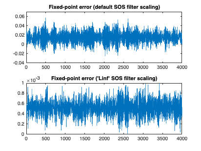
Infinity-norm SOS scaling often produces outputs with lower error.
fig1 = figure;
subplot(3,1,1);
plot(out_1);
title('Floating-point filter output');
subplot(3,1,2);
plot(out_4);
title('Fixed-point (Linf-norm SOS) filter output');
subplot(3,1,3);
plot(out_1 - double(out_4));
axis([0 4000 0 1e-3]);
title('Error');

fig2 = figure;
subplot(2,1,1);
plot(out_1 - double(out_3));
axis([0 4000 -4e-2 7e-2]);
title('Fixed-point error (default SOS filter scaling)');
subplot(2,1,2);
plot(out_1 - double(out_4));
axis([0 4000 0 1e-3]);
title('Fixed-point error (''Linf'' SOS filter scaling)');
close(fig1); % clean up
close(fig2); % clean up
Summary
We have outlined a procedure to convert a floating-point IIR filter to a fixed-point implementation. The dsp.BiquadFilter objects of the DSP System Toolbox™ are equipped with Simulation Minimum and Maximum instrumentation capabilities that help the Fixed-Point Converter App automatically and dynamically scale internal filter signals. In addition, various 'fvtool' and spectrumAnalyzer analyses provide tools to the user to perform verifications at each step of the process.
You can also select a web site from the following list:
Americas
- América Latina (Español)
- Canada (English)
- United States (English)
Europe
- Belgium (English)
- Denmark (English)
- Deutschland (Deutsch)
- España (Español)
- Finland (English)
- France (Français)
- Ireland (English)
- Italia (Italiano)
- Luxembourg (English)
- Netherlands (English)
- Norway (English)
- Österreich (Deutsch)
- Portugal (English)
- Sweden (English)
- Switzerland
- United Kingdom (English)