Satellite Conjunction Finder
This example shows how to find potential events of close proximity or conjunctions of two satellites.
To find potential upcoming conjunctions, the example uses the SOCRATES tool, available from the CelesTrak™ web site. SOCRATES generates lists of upcoming conjunctions using two-line elements (TLEs) that are stored in a text file for easy loading into the satellite scenario object. The conjunction lists generated by SOCRATES are used with permission from CelesTrak.
As a general workflow:
To find windows when the two satellites pass within a specified control distance, such as 200 km, the example uses the simulation capability within the
satelliteScenarioobject. This search requires a sample time along the orbit of about 20 seconds.Use
fzerowith a gradient function to find the time of closest approach for each window.Visualize the output and confirm the same conjunction as
SOCRATEShas been located.
Disclaimer - Do not use publicly available TLEs for operational conjunction assessment prediction. This example is provided for informational purposes only. Satellite operators should contact the 18th Space Defense Squadron for data and analysis to support operational satellites.
Choose a Conjunction Scenario
The main page of SOCRATES provides two conjunction lists, the top 10 conjunctions by either maximum probability or maximum range. Clicking on a list shows a table of the conjunctions with the satellite names, date and time of closest approach (TCA), maximum probability of collision, and relative velocity. Each entry in the table has a button to display the TLEs in a separate window. You can copy these TLEs into a text file. An example of a copied conjunction follows.
type Conjunction_Starlink1079_CZ2DDeb.txtSTARLINK-1079 1 44937U 20001Z 22272.52136386 -.00000745 00000+0 -31120-4 0 9997 2 44937 53.0548 210.2777 0001443 83.0631 277.0522 15.06393387150649 CZ-2D DEB 1 43406U 12073D 22272.74034628 .00008296 00000+0 83006-3 0 9993 2 43406 97.9471 196.5364 0090895 225.9886 133.3815 14.88613293478469
Conjunction data from SOCRATES:
44937 STARLINK-1079 [+], Days since epoch: 3.81743406 CZ-2D DEB [-], Days since Epoch: 3.598Max Probability 1.363E-02Dilution Threshold (km) 0.004Min Range (km) 0.017Relative Velocity (km/sec) 5.861Start (UTC) 2022 Oct 03 08:06:48.977TCA (UTC) 2022 Oct 03 08:06:49.830Stop (UTC) 2022 Oct 03 08:06:50.683
Parameters for the conjunction list are:
Data current as of 2022 Sep 30 08:05 UTC
Computation Interval: Start = 2022 Sep 30 00:00:00.000, Stop = 2022 Oct 07 00:00:00.000
Computation Threshold: 5.0 km
Considering: 9,400 Primaries, 23,748 Secondaries (115,200 Conjunctions)
This example uses satelliteScenario to validate the time and distance of closest approach as reported by SOCRATES. For this particular conjunction example, notice that the satellites have two close passes in seven days.
This example provides two StarLink satellite TLE text files and one ORSTED satellite and Iridrium33 satellite TLE text file retrieved from SOCRATES. The two StarLink satellite TLE text files produce over 200 coarse conjunction windows, as the satellites pass close to each other every half orbit. This analysis takes some time to run with a closest approach of 10 m found. The ORSTED and Iridium 33 TLE text file produces nearly 20 coarse windows, with a closest distance of 26 m.
From the list, choose a TLE text file to run.
tleFile =
"Conjunction_Starlink1079_CZ2DDeb.txt"
tleFile = "Conjunction_Starlink1079_CZ2DDeb.txt"
Load the Satellite Elements into a Scenario Object
Load the TLEs directly into the satelliteScenario using a plain text file. TLEs are a text representation of the satellite orbital elements for use with the SGP4 or SDP4 propagators.
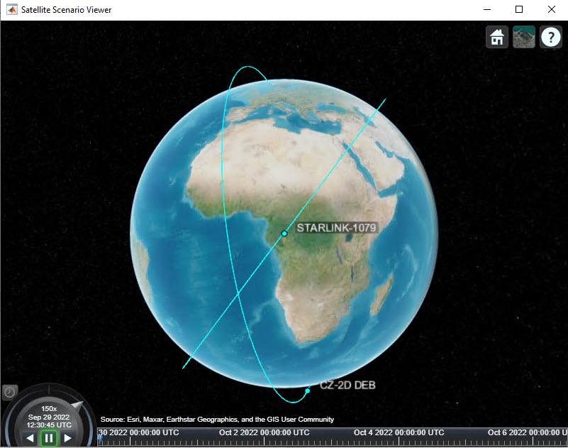
sc  = satelliteScenario;
satellites = satellite(sc,tleFile);
v = satelliteScenarioViewer(sc);
v.PlaybackSpeedMultiplier = 150;
Here is a screenshot of the viewer for the first example. The controls are on the bottom left. We can see that the orbits cross at a similar altitude.
Find Windows When the Satellites Pass Within a Specified Distance
Measure the time it takes to find all the windows with seven days, the standard time period to check for conjunctions according to the NASA handbook [1]. A sample time of 20 seconds is sufficient for LEO satellites.
startTime_init = sc.StartTime;
sc.StopTime  = startTime_init + days(7);
sc.SampleTime = 20;
Get the satellite position data and associated times using the aer function. This method of the Satellite class computes azimuth angle, elevation angle, and the range of a satellite and another object. In this case, the other object is the other satellite.
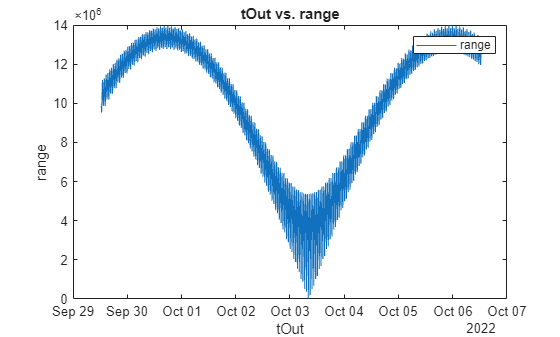
[~,~,range,tOut] = aer(satellites(1),satellites(2));
Then, plot the range versus tOut.
% Create plot of tOut and range
h2 = plot(tOut,range,"DisplayName","range");

% Add xlabel, ylabel, title, and legend
xlabel("tOut")
ylabel("range")
title("tOut vs. range")
legend
Compute the distance between the two satellite positions. Determine the indices of the range when the satellite are closer than the target of 200 km. Then, use a for loop to find the times when this relative distance is less than a target of 200 km. The diff function finds the gaps in between the found points. If the value is 1, the points are adjacent to the window and the stop time can be extended. To create a window of time, add the ephemeric point before and after the found points.
dMinTarget = 200e3;
kCloseIdx  = find(range<dMinTarget);
dW         = [0 diff(kCloseIdx)];
kWindow    = zeros(2,length(kCloseIdx));
j          = 1;
for m = 1:length(dW)
  if dW(m)~=1
    % single point window
    kWindow(1,j) = max(1,kCloseIdx(m)-1);
    kWindow(2,j) = kCloseIdx(m)+1;
    j = j+1;
  elseif j>1
    % update window end as long as diff==1
    kWindow(2,j-1) = kCloseIdx(m)+1;
  end
end
Since any found multiple-point windows reduces the number of windows below the number of close points, limit the output to the windows found. The resulting number of found windows is printed to the command line.
kWindow = kWindow(:,1:j-1);
fprintf("%d windows found for dMin = %g km\n",size(kWindow,2),dMinTarget*1e-3);
2 windows found for dMin = 200 km
To get the datetime of the windows from output time array, use the window indices. Display windows to check the results. The windows are about a minute long.
windows = tOut(kWindow);
if size(windows,2)>=3
  disp(windows(:,1:3)')
else
disp(windows')
end
   03-Oct-2022 08:06:05   03-Oct-2022 08:07:25
   03-Oct-2022 08:54:25   03-Oct-2022 08:55:05
Test the Gradient Function over One Window
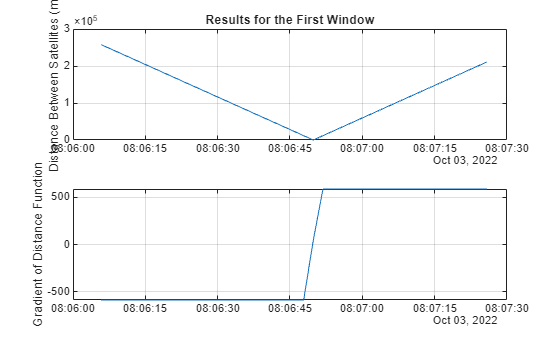
To find the point of closest approach, look for the cost to change sign over the window. Using a for loop, call the gradient function for an array of times within the first window using a timestep of 2 seconds. The gradientScenario function is in a separate file. At each time step, compute a duration in days from the scenario start time. Store the gradient and distance between the satellites.
window = windows(:,1);
tVec   = window(1):seconds(2):window(2);
dRDot  = zeros(size(tVec));
dR     = zeros(size(tVec));
for k = 1:length(tVec)
  delT = days(tVec(k) - sc.StartTime);
  [dRDot(k),dR(k)] = gradientScenario(delT,satellites(1),satellites(2),sc.StartTime);
end
Use figure and subplot to create a plot of both the minimum distance and the gradient function output. Confirm the sign change at the point of closest approach.
figure('name','Gradient Test over One Window')
subplot(211)
plot(tVec,dR)
grid on
ylabel('Distance Between Satellites (m)')
title('Results for the First Window')
subplot(212)
plot(tVec,dRDot)
grid on
ylabel('Gradient of Distance Function')
Search the Windows for the Closest Approach
Pass in the start and stop time of the window to give fzero a range. The days function converts the datetime array to a double. Use an anonymous function to pass the satelliteScenario object to the gradient function. To measure the elapsed time of the for loop, use tic and toc. For some satellite pairs, the elapsed time might exceed a minute.
tMin = zeros(1,size(windows,2));
dRs  = zeros(1,size(windows,2));
h = waitbar(0,'Please wait, iterating over windows...');
tic
for k = 1:size(windows,2)
  tMin(k) = fzero(@(t) gradientScenario(t,satellites(1),satellites(2),sc.StartTime),days(windows(:,k)-sc.StartTime));
  [~,dRs(k)] = gradientScenario(tMin(k),satellites(1),satellites(2),sc.StartTime);
  waitbar(k/size(windows,2),h);
end
close(h)
toc
Elapsed time is 1.134183 seconds.
Find the minimum distance of all the windows and report the time of closest approach found. The distance is displayed in meters.
[rMin,iMin] = min(dRs);
tCA = sc.StartTime + tMin(iMin);
disp(tCA)
03-Oct-2022 08:06:49
disp(dRs(iMin))
17.1728
Verify the relative velocity between the satellites from SOCRATES using the states function and the time of closest approach. The velocity is in m/s.
[~,vel] = states(satellites,tCA); % satellite velocity in m/s
dV = vecnorm(vel(:,:,1) - vel(:,:,2));
disp(dV)
5.8613e+03
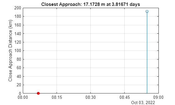
To plot the resulting close passes, use the stem function. Mark the closest approach in red. Notice that the result is the same as that reported by SOCRATES.
figure('name','ConjunctionDetection')
stem(sc.StartTime + tMin,dRs*1e-3)
ylabel('Close Approach Distance (km)')
title(sprintf('Closest Approach: %g m at %g days',rMin,tMin(iMin)))
hold on; grid on;
stem(sc.StartTime + tMin(iMin),rMin*1e-3,'filled','r') % mark the closest approach
In summary, it is a two-step process to find the closest approach of one satellite to another during a seven day time window.
Find windows of close approach using a coarse filter with distance metric.
Find the closest pass within each window using
fzero.
This two-step method can replicate the conjunctions reported by the SOCRATES website:
Time of closest approach (TCA)
Distance between the satellites
Relative velocity
Update the Scenario Around the Found Conjunction
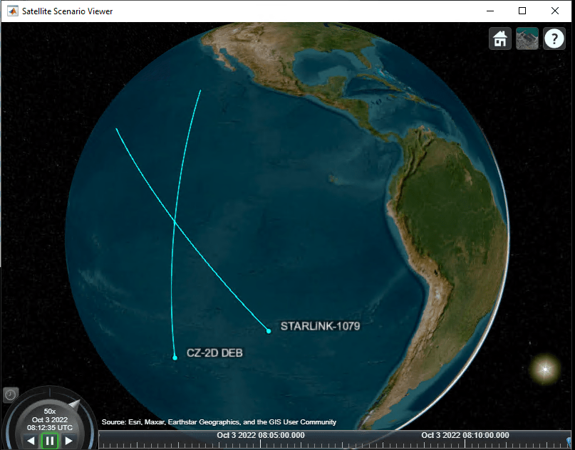
Now that we have the time of closest approach, update the simulation start and stop times to be a few minutes more or less. Use the play function to run the simulation.
Here is a screenshot of the conjunction from our first example.
sc.StartTime = tCA - days(0.004);
sc.StopTime = tCA + days(0.004);
v.PlaybackSpeedMultiplier = 50;
campos(v,-10.5641,-98.9574,9.1906e6);
play(sc);
References
[1] NASA Spacecraft Conjunction Assessment and Collision Avoidance Best Practices Handbook, December 2020, NASA/SP-20205011318, https://nodis3.gsfc.nasa.gov/OCE_docs/OCE_50.pdf.