Design and Analyze Cassegrain Antenna

This example shows how to create and analyze a cassegrain antenna. A typical parabolic antenna consists of a parabolic reflector with a small feed antenna at its focus. Parabolic reflectors used in dish antennas have a large curvature and short focal length to reduce the length of the supports required to hold the feed structure. In more complex designs, such as the cassegrain antenna, a sub-reflector is used to direct the energy into the parabolic reflector from a feed antenna located away from the primary focal point. Cassegrain provides an option to increase focal length thereby reducing side lobes. Such type of antennas can be used in satellite communications as well as Astronomy and other emerging modes of communications.

Define Parameters

A Cassegrain antenna typically consists of three components: a parabolic main reflector, a hyperbolic sub-reflector, and an exciter. Define the parameters such as radius and focal length for main and sub-reflectors as below.

Rp = Radius of main reflector

fp = Focal length of main reflector

Rsub = Radius of sub-reflector

fsub = Focal length of sub-reflector

Rp = 0.3175;
fp = 0.2536;
Rsub = 0.033;
fsub = 0.1416;

Model Cassegrain Antenna

Focus of main reflector and the near focus of hyperbolic sub-reflector coincides. The energy is directed from the sub-reflector towards main reflector. The parabolic reflector converts a spherical wavefront into a plane wavefront as the energy directed towards it appears to be coming from focus. Use the cassegrain object from the antenna catalog to create a Cassegrain antenna with specified geometric parameters.

ant = cassegrain(Radius=[Rp Rsub], FocalLength=[fp fsub]);
show(ant)

Define Exciter Element

The default exciter for cassegrain object is a conical horn antenna. It is designed at a frequency which gives the desired performance. Orient it towards the sub-reflector. Choose the aperture diameter analytically to give the desired co-planar pattern beam width.

Exciter = design(hornConical,17.7e9);
Exciter.FeedWidth = 3.4e-3;
Exciter.Tilt = 270;
Exciter.TiltAxis = [0 1 0]; 
show(Exciter)

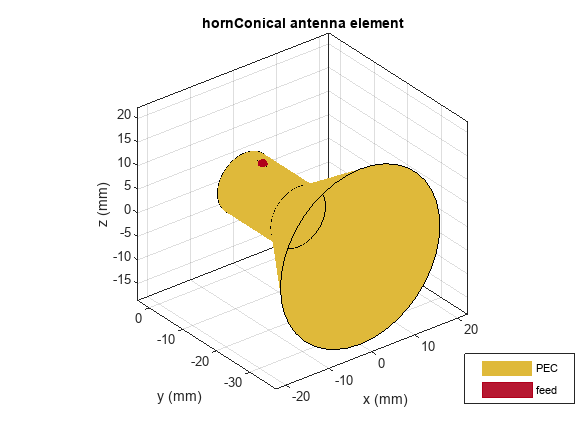
Solve Structure

Default Cassegrain antenna uses PO solver for main reflector and MoM solver for sub-reflector and exciter. Diameter of main reflector is 39$\lambda$ (where $\lambda$ is the operating wavelength) and that of sub reflector is 4$\lambda$. Solvers are used according to the size of main reflector and sub-reflector. Typically, if the diameter of sub-reflector is greater than 5$\lambda$, then it is recommended to use PO solver for it. Normally the expected diameter of sub-reflector has to be less than 20% of main reflector to minimize the blockage by the sub-reflector.

Default Cassegrain antenna generates more number of triangles, so it can be meshed manually for different mesh edge lengths for the required numbers of triangular generation. This solves the structure quickly, but the gain decreases compared to default in such cases. Mesh can be controlled for exciters and reflectors separately with different mesh edge lengths.

ant = cassegrain;
ant.Exciter = design(hornConical,17.7e9);
ant.Exciter.Tilt = 270;
[~] = mesh(ant,MaxEdgeLength=15e-3);

Plot Radiation Pattern

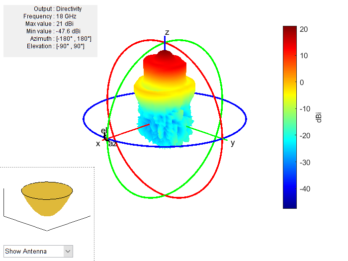
Plot the radiation pattern of Cassegrain antenna at 18GHz. The expected pattern need to generate a pencil like beam with less spill over and minor lobe radiation.

figure
pattern(ant,18e9);

Compare the radiation pattern of this Cassegrain configuration with parabolic reflector configuration which does not have a sub-reflector. The Cassegrain configuration has more directivity than a parabolic reflector for the same exciter element.

ant = reflectorParabolic(Radius=0.3175);
ant.Exciter = design(hornConical,17.7e9);
ant.Exciter.Tilt = 90;
figure
pattern(ant,18e9);

Plot S-parameters and Impedance

Plot the S-parameters and impedance of cassegrain antenna over a frequency range of 18 GHz to 18.8 GHz. It provides a bandwidth of about 100MHz and the structure resonates at 18.51 GHz.

ant = cassegrain;
s = sparameters(ant,linspace(18e9,18.8e9,25));
figure
rfplot(s);

figure
impedance(ant,linspace(18e9,18.8e9,25));

Visualize Current Distribution

Visualize the current distribution of Cassegrain antenna at a specified frequency.

current(ant,18e9,Scale="log10");

Use Different Exciters with Tilts

Several other elements of the type horn and waveguide are supported as exciters for the Cassegrain antenna. Exciter can be tilted in the required direction based on the need. Use horn object as the exciter, orient it towards sub-reflector and plot the radiation pattern at 18GHz.

Exciter = design(horn,16.2e9);
Exciter.Tilt = 270;
Exciter.TiltAxis = [0 1 0]; 
ant.Exciter = Exciter;
show(ant)

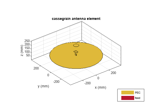
figure
pattern(ant,18e9);

Conclusion

The Cassegrain antenna configuration enhances performance by orienting the feed antenna to direct signals forward, unlike front-fed dish antennas. This orientation reduces side lobes and leverages a dual-reflector system to tailor the radiation pattern for maximum antenna performance.

References

[1] Dandu, Obulesu. “Optimized Design of Axially Symmetric Cassegrain Reflector Antenna Using Iterative Local Search Algorithm.” National Institute of Technology, Rourkela, 2013. http://ethesis.nitrkl.ac.in/5438/1/211EE1116.pdf.