Reflector Backed Equiangular Spiral
The spiral antenna is an inherently broadband, and bidirectional radiator. This example will analyze the behavior of an equiangular spiral antenna backed by a reflector [1]. The spiral and the reflector are Perfect Electric Conductors (PEC).
Spiral and Reflector Parameters
The spiral antenna parameters and reflector dimensions are provided in [1]. The design frequency range is 4-9 GHz and the analysis frequency range will span 3-10 GHz.
a = 0.35;
rho = 1.5e-3;
phi_start = -0.25*pi;
phi_end = 2.806*pi;
R_in = rho*exp(a*(phi_start + pi/2));
R_out = rho*exp(a*(phi_end + pi/2));
gndL = 167e-3;
gndW = 167e-3;
spacing = 7e-3;
Create Equiangular Spiral Antenna
Create an equiangular spiral antenna using the defined parameters.
sp = spiralEquiangular;
sp.GrowthRate = a;
sp.InnerRadius = R_in;
sp.OuterRadius = R_out;
figure
show(sp)
title("Equiangular Spiral Antenna Element");
Create a reflector, and assign the spiral antenna as its exciter. Adjust the spacing between the reflector and spiral to be 7 mm. The first-pass analysis will be with an infinitely large groundplane. To do this, assign the groundplane length and/or width to inf.
rf = reflector;
rf.GroundPlaneLength = inf;
rf.GroundPlaneWidth = inf;
rf.Exciter = sp;
rf.Spacing = spacing;
figure
show(rf)
title("Equiangular Spiral Antenna Element Over an Infinite Reflector");
Impedance Analysis of Spiral with and without Infinite Reflector
Define a frequency range for the impedance analysis. Keep the frequency range sampling coarse to get an overall idea of the behavior. A detailed analysis will follow. Analyze the impedance of both antennas: the spiral antenna in free space and the antenna with the infinite reflector.
freq = linspace(3e9,10e9,31);
figure
impedance(sp,freq)

figure
impedance(rf,freq);

The impedance for the spiral without the reflector is smooth in both resistance and reactance. The resistance holds steady around the 184 value while the reactance although slightly capacitive, does not show any drastic variations. However, introducing an infinitely large reflector at a spacing of 7mm disturbs this smooth behavior for both the resistance and reactance.
Make Reflector Finite
Change the reflector to be of finite dimensions by using the dimensions specified earlier as per [1].
rf.GroundPlaneLength = gndL;
rf.GroundPlaneWidth = gndW;
show(rf)
title("Equiangular Spiral Antenna Element Over Finite Reflector");
Mesh Different Parts Independently
To analyze the behavior of the spiral antenna backed by the finite-size reflector, mesh the antenna and reflector independently. The highest frequency in the analysis is 10 GHz, which corresponds to a of 3 cm. Mesh the spiral with a maximum edgelength of 2 mm (lower than = 3mm at 10 GHz). This requirement is relaxed for the reflector which is meshed with a maximum edge length of 8mm (slightly lower than = 10cm at 3 GHz).
ms_new = mesh(rf.Exciter,MaxEdgeLength=0.002)
mr_new = mesh(rf,MaxEdgeLength=0.008)
Impedance Analysis of the Spiral Antenna with the Finite Reflector
Run the following code snippet at the prompt in the command window to create an accurate impedance plot for the finite reflector shown in the figure that follows. The impedance behavior typical for the infinitely large reflector is also observed for the finite reflector.
fig1 = figure;
impedance(rf,linspace(3e9,10e9,200));
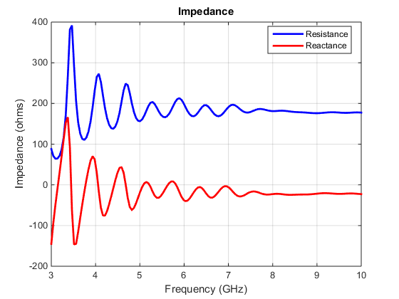
Fig. 1: Input impedance of the spiral with metal(PEC) reflector
Surface Currents on Reflector-Backed Spiral Antenna
Run the following code snippet at the prompt in the Command Window to recreate the current distribution plots shown in the figure that follows. Since the design frequency band is 4 - 9 GHz, pick the two band edge frequencies for observing the surface currents on the spiral antenna. From the impedance analysis, the presence of multiple resonances at the lower end of the design frequency band, should manifest itself in the surface currents at 4 GHz.
fig2 = figure;
current(rf,4e9)
view([0 90])
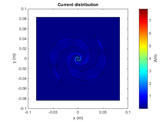
Fig. 2: Surface current density at 4 GHz
At first glance, the surface current density plot might appear to not reveal any information. To explore further, use the colorbar on the right of the plot. This colorbar allows you to adjust the color scale interactively. To interact with the colorbar, move the mouse pointer on the colorbar, right-click and select Interactive Colormap Shift. To adjust the scale, move the mouse pointer to an area within the colorbar boundary, click, and drag. To adjust the range of values, move the mouse pointer outside the colorbar boundary and hover over the numeric tick marks on the colorbar or between the tick spacings, click and drag. This approach generates the following figure, which indicates presence of standing waves at 4GHz. The arrows on the plot are added separately to highlight the local current minima.
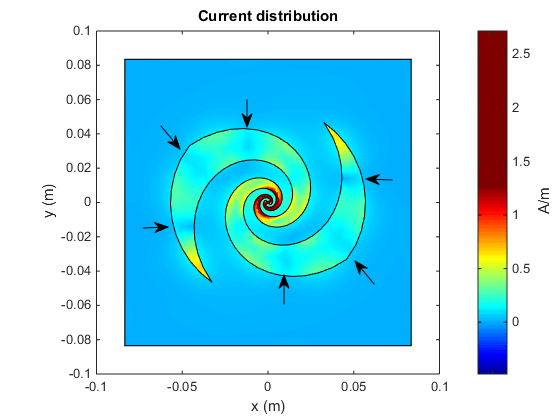
Fig. 3: Surface current density at 4 GHz after adjusting the dynamic range using the colorbar
Plot the current density on the spiral antenna at 9 GHz.
fig4 = figure;
current(rf,9e9)
view([0 90])
As in the previous case, we use the colorbar to adjust the scale to be similar and observe a current flow that is free of any standing waves.
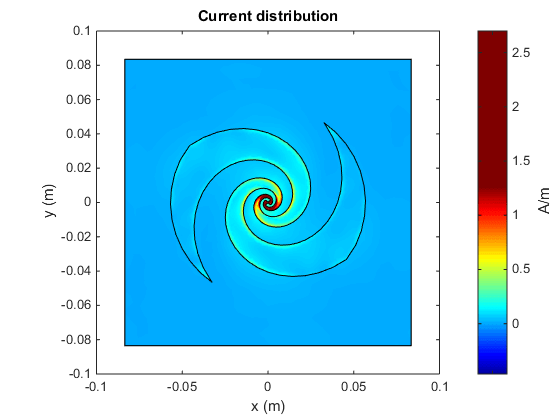
Fig. 4: Surface current density at 9 GHz
Calculate and Plot Axial Ratio
The spiral antenna radiates circularly polarized waves. The axial ratio (AR) in a given direction quantifies the ratio of two orthogonal field components radiated in a circularly polarized wave. An axial ratio of infinity, implies a linearly polarized wave. When the axial ratio is 1, the radiated wave has pure circular polarization. Values greater than 1 imply elliptically polarized waves. Run the following code snippet at the prompt in the command window to recreate the axial ratio plot at broadside shown in the figure that follows. Note that the calculated axial ratio values are in dB, 20log10(AR). To compare the effect of the reflector, calculate the axial ratio for the spiral antenna with and without the reflector.
AR_spiral = zeros(size(freq));
AR_reflector = zeros(size(freq));
for i = 1:numel(freq)
 AR_spiral(i) = axialRatio(rf.Exciter,freq(i),0,90);
 AR_reflector(i) = axialRatio(rf,freq(i),0,90);
end
Plot the axial ratio of the spiral antenna with and without the reflector.
fig5 = figure;
plot(freq/1e9,AR_spiral,LineWidth=2);
hold on
plot(freq./1e9,AR_reflector,'m',LineWidth=2);
grid on
ax1 = fig5.CurrentAxes;
ax1.YTickLabelMode = 'manual';
ax1.YLim = [0 20];
ax1.YTick = 0:2:20;
ax1.YTickLabel = cellstr(num2str(ax1.YTick'));
xlabel("Frequency (GHz)")
ylabel("AR (dB)")
title("Frequency Response of Axial Ratio")
legend("Without reflector","With reflector");
The axial ratio plot of the spiral without the reflector shows that across the design frequency band, the spiral antenna radiates a nearly circularly polarized wave. The introduction of the reflector close to the spiral antenna degrades the circular polarization.
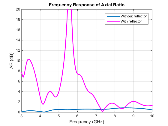
Fig. 5: Axial ratio at broadside in dB with and without reflector backing as a function of frequency [1]
Conclusion
The spiral antenna by itself has a broad impedance bandwidth and produces a bi-directional radiation pattern. It also produces a circularly polarized wave across the bandwidth. A unidirectional beam can be created by using a backing structure like reflector or cavity. Maintaining the desired performance when using a traditional metallic/PEC reflector, especially at small separation distances is difficult [1].
Reference
[1] Nakano, Hisamatsu, Katsuki Kikkawa, Norihiro Kondo, Yasushi Iitsuka, and Junji Yamauchi. “Low-Profile Equiangular Spiral Antenna Backed by an EBG Reflector.” IEEE Transactions on Antennas and Propagation 57, no. 5 (May 2009): 1309–18. https://doi.org/10.1109/TAP.2009.2016697.