Wideband Blade Dipole Antenna and Array
This example shows the analysis of a blade dipole as a single element and in a 2-by-2 array with emphasis on its wideband behavior.
The Blade Dipole
Strip dipoles or the cylindrical counterparts have a significant capacitive component to its impedance and typically possess a narrow impedance bandwidth. It is well known that widening the dipole or thickening the cylindrical cross-sections makes it easier to impedance match over a broader frequency range [1]. These wide dipoles, are known as blade dipoles. We will model such a blade dipole in this example [2].
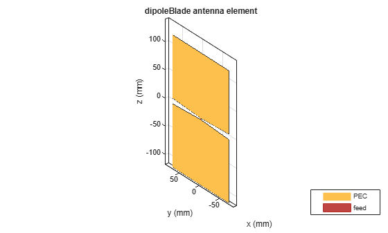
L = 117e-3;         % Total half-length of blade dipole
W = 140e-3;         % Width of blade dipole
Ld = 112e-3;        % Half-length excluding impedance match taper
fw = 3e-3;          % Feed width
g = 3e-3;           % Feed gap

bladeDipole = dipoleBlade(Length=L, Width=W);
The blade dipole consists of two identical metallic arms that include a tapered section close to the feed. The tapered section ensures a better impedance match to 50.
figure
show(bladeDipole)
Calculate Reflection Coefficient of Blade Dipole
A good way to understand the quality of impedance matching, in this case to 50, is to study the reflection coefficient of the antenna. We choose the frequency range of 200 MHz to 1.2 GHz and calculate the S-parameters of the antenna.
fmin = 0.2e9;
fmax = 1.2e9;
Nfreq = 21;
freq = linspace(fmin,fmax,Nfreq);
s_blade = sparameters(bladeDipole,freq);
Compare with Thin Dipole
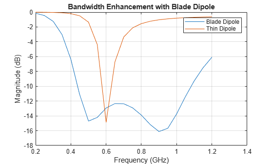
To understand the difference between the performance of a blade dipole and of a traditional thin dipole, create a typical dipole from the Antenna Toolbox library with the same total length as the blade dipole but with the width being the same as the feedwidth, i.e. 3mm. Calculate and plot the reflection coefficient of both dipoles.
thinDipole = dipole;
thinDipole.Length = 2*L;
thinDipole.Width = fw;
s_thin = sparameters(thinDipole,freq);
figure
rfplot(s_blade,1,1);
hold on
rfplot(s_thin,1,1)
legend("Blade Dipole","Thin Dipole")
title("Bandwidth Enhancement with Blade Dipole")
Build 2-by-2 Array of Blade Dipoles on Infinite GroundPlane
Such blade dipoles can be used as building blocks for modular arrays [2].
Create blade dipole backed by an infinite reflector
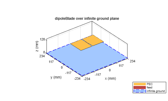
Assign the blade dipole as a the exciter to a reflector of infinite extent. The dipole is positioned on the X-Y plane (z=0).
bladeDipole.Tilt = 90;
bladeDipole.TiltAxis = [0 1 0];
ref = reflector;
ref.Exciter = bladeDipole;
ref.GroundPlaneLength = inf;
ref.GroundPlaneWidth = inf;
ref.Spacing = 120e-3;
figure
show(ref)
Create rectangular array with the reflector backed dipole
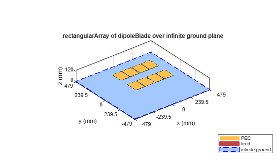
Make a 2-by-2 rectangular array with the reflector backed blade dipole. The spacing between elements are chosen for the center of the band. This might introduce grating lobes since the spacing becomes approximately 0.81 at 1 GHz. However, for non-scanning applications this larger spacing should not cause problems.
ref_array = rectangularArray;
ref_array.Element = ref;
ref_array.RowSpacing = 245e-3;
ref_array.ColumnSpacing = 245e-3;
figure
show(ref_array);
Calculate Active Reflection Coefficient
For a small 2-by-2 array, each element experiences the same environment. Therefore the active reflection coefficient of any of the elements should suffice to understand the matching performance.
s_array = sparameters(ref_array,freq);
figure
rfplot(s_array,1,1)
title("Active Element Reflection Coefficient")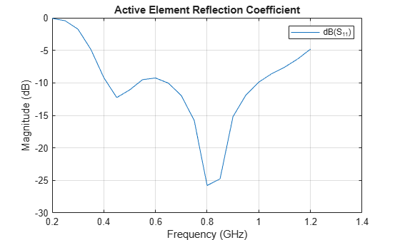
The blade dipole in a 2-by-2 array continues to show broadband performance. The bandwidth is approximately 2.6:1, measured as the ratio of the highest to the lowest frequency at which the reflection coefficient curve crosses -10 dB.
References
[1] C. A. Balanis, Antenna Theory. Analysis and Design, Wiley, New York, 3rd Edition, 2005.
[2] V. Iyer, S. Makarov, F. Nekoogar, "On wideband modular design of small arrays of planar dipoles," IEEE Antennas and Propagation Society International Symposium (APSURSI), pp.1-4, 11-17 July 2010.