Fixed-Structure Autopilot for a Passenger Jet
This example shows how to use slTuner and systune to tune the standard configuration of a longitudinal autopilot. We thank Professor D. Alazard from Institut Superieur de l'Aeronautique et de l'Espace for providing the aircraft model and Professor Pierre Apkarian from ONERA for developing the example.
Aircraft Model and Autopilot Configuration
The longitudinal autopilot for a supersonic passenger jet flying at Mach 0.7 and 5000 ft is depicted in Figure 1. The autopilot main purpose is to follow vertical acceleration commands  issued by the pilot. The feedback structure consists of an inner loop controlling the pitch rate
  and an outer loop controlling the vertical acceleration
  . The autopilot also includes a feedforward component and a reference model
  that specifies the desired response to a step command . Finally, the second-order roll-off filter
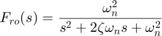
is used to attenuate noise and limit the control bandwidth as a safeguard against unmodeled dynamics. The tunable components are highlighted in orange.
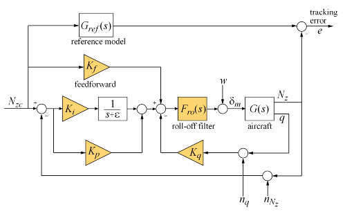
Figure 1: Longitudinal Autopilot Configuration.
The aircraft model  is a 5-state model, the state variables being the aerodynamic speed
  (m/s), the climb angle
  (rad), the angle of attack
  (rad), the pitch rate (rad/s), and the altitude
  (m). The elevator deflection
  (rad) is used to control the vertical load factor . The open-loop dynamics include the oscillation with frequency and damping ratio
  = 1.7 (rad/s) and
  = 0.33, the phugoid mode = 0.64 (rad/s) and = 0.06, and the slow altitude mode
  = -0.0026.
load ConcordeData G
bode(G,{1e-3,1e2}), grid
title('Aircraft Model')
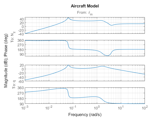
Note the zero at the origin in . Because of this zero, we cannot achieve zero steady-state error and must instead focus on the transient response to acceleration commands. Note that acceleration commands are transient in nature so steady-state behavior is not a concern. This zero at the origin also precludes pure integral action so we use a pseudo-integrator  with
with  = 0.001.
Tuning Setup
When the control system is modeled in Simulink®, you can use the slTuner interface to quickly set up the tuning task. Open the Simulink model of the autopilot.
open_system('rct_concorde')
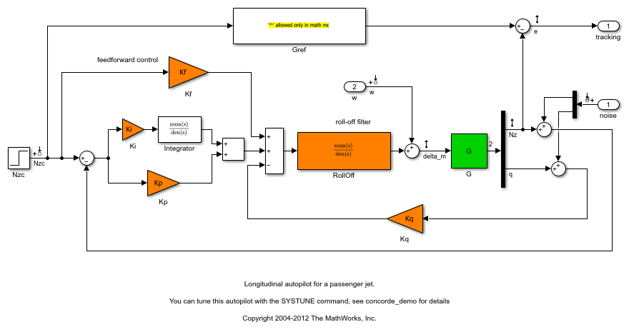
Configure the slTuner interface by listing the tuned blocks in the Simulink model (highlighted in orange). This automatically picks all Linear Analysis points in the model as points of interest for analysis and tuning.
ST0 = slTuner('rct_concorde',{'Ki','Kp','Kq','Kf','RollOff'});
This also parameterizes each tuned block and initializes the block parameters based on their values in the Simulink model. Note that the four gains Ki,Kp,Kq,Kf are initialized to zero in this example. By default the roll-off filter  is parameterized as a generic second-order transfer function. To parameterize it as
create real parameters  , build the transfer function shown above, and associate it with the
 RollOff block.
wn = realp('wn', 3);               % natural frequency
zeta = realp('zeta',0.8);          % damping
Fro = tf(wn^2,[1 2*zeta*wn wn^2]); % parametric transfer function

setBlockParam(ST0,'RollOff',Fro)   % use Fro to parameterize "RollOff" block
Design Requirements
The autopilot must be tuned to satisfy three main design requirements:
1. Setpoint tracking: The response to the command should closely match the response of the reference model:
This reference model specifies a well-damped response with a 2 second settling time.
2. High-frequency roll-off: The closed-loop response from the noise signals to should roll off past 8 rad/s with a slope of at least -40 dB/decade.
3. Stability margins: The stability margins at the plant input should be at least 7 dB and 45 degrees.
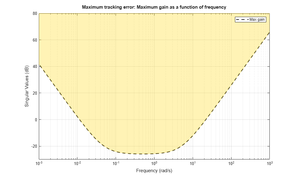
For setpoint tracking, we require that the gain of the closed-loop transfer from the command to the tracking error  be small in the frequency band [0.05,5] rad/s (recall that we cannot drive the steady-state error to zero because of the plant zero at s=0). Using a few frequency points, sketch the maximum tracking error as a function of frequency and use it to limit the gain from to .
Freqs = [0.005 0.05 5 50];
Gains = [5 0.05 0.05 5];
Req1 = TuningGoal.Gain('Nzc','e',frd(Gains,Freqs));
Req1.Name = 'Maximum tracking error';
The TuningGoal.Gain constructor automatically turns the maximum error sketch into a smooth weighting function. Use viewGoal to graphically verify the desired error profile.
viewGoal(Req1)
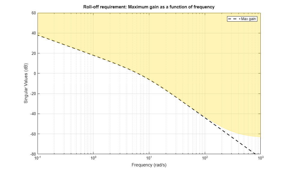
Repeat the same process to limit the high-frequency gain from the noise inputs to and enforce a -40 dB/decade slope in the frequency band from 8 to 800 rad/s
Freqs = [0.8 8 800];
Gains = [10 1 1e-4];
Req2 = TuningGoal.Gain('n','delta_m',frd(Gains,Freqs));
Req2.Name = 'Roll-off requirement';

viewGoal(Req2)
Finally, register the plant input as a site for open-loop analysis and use TuningGoal.Margins to capture the stability margin requirement.
addPoint(ST0,'delta_m')

Req3 = TuningGoal.Margins('delta_m',7,45);
Autopilot Tuning
We are now ready to tune the autopilot parameters with systune. This command takes the untuned configuration ST0 and the three design requirements and returns the tuned version ST of ST0. All requirements are satisfied when the final value is less than one.
[ST,fSoft] = systune(ST0,[Req1 Req2 Req3]);
Final: Soft = 0.965, Hard = -Inf, Iterations = 86
Use showTunable to see the tuned block values.
showTunable(ST)
Block 1: rct_concorde/Ki =

  D =
             u1
   y1  -0.02989

Name: Ki
Static gain.

-----------------------------------

Block 2: rct_concorde/Kp =

  D =
              u1
   y1  -0.009776

Name: Kp
Static gain.

-----------------------------------

Block 3: rct_concorde/Kq =

  D =
            u1
   y1  -0.2863

Name: Kq
Static gain.

-----------------------------------

Block 4: rct_concorde/Kf =

  D =
             u1
   y1  -0.02259

Name: Kf
Static gain.

-----------------------------------

wn = 4.81
-----------------------------------
zeta = 0.513
To get the tuned value of , use getBlockValue to evaluate Fro for the tuned parameter values in ST:
Fro = getBlockValue(ST,'RollOff');
tf(Fro)
ans =

          23.16
  ---------------------
  s^2 + 4.941 s + 23.16

Continuous-time transfer function.
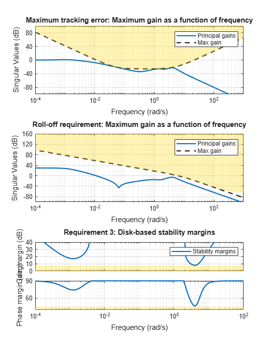
Finally, use viewGoal to graphically verify that all requirements are satisfied.
figure('Position',[100,100,550,710])
viewGoal([Req1 Req2 Req3],ST)
Closed-Loop Simulations
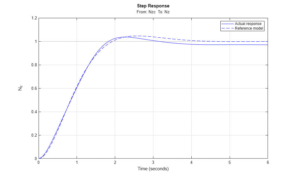
We now verify that the tuned autopilot satisfies the design requirements. First compare the step response of with the step response of the reference model . Again use getIOTransfer to compute the tuned closed-loop transfer from Nzc to Nz:
Gref = tf(1.7^2,[1 2*0.7*1.7 1.7^2]);    % reference model

T = getIOTransfer(ST,'Nzc','Nz');  % transfer Nzc -> Nz

figure, step(T,'b',Gref,'b--',6), grid,
ylabel('N_z'), legend('Actual response','Reference model')
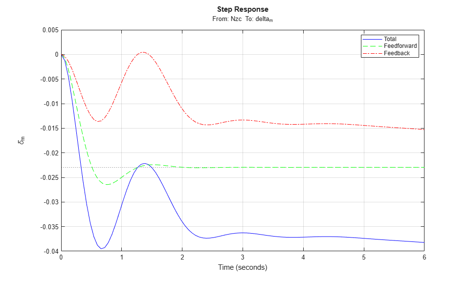
Also plot the deflection and the respective contributions of the feedforward and feedback paths:
T = getIOTransfer(ST,'Nzc','delta_m');  % transfer Nzc -> delta_m
Kf = getBlockValue(ST,'Kf');            % tuned value of Kf
Tff = Fro*Kf;         % feedforward contribution to delta_m

step(T,'b',Tff,'g--',T-Tff,'r-.',6), grid
ylabel('\delta_m'), legend('Total','Feedforward','Feedback')
Finally, check the roll-off and stability margin requirements by computing the open-loop response at .
OL = getLoopTransfer(ST,'delta_m',-1); % negative-feedback loop transfer
margin(OL);
grid;
xlim([1e-3,1e2]);
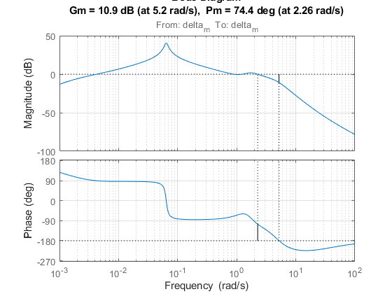
The Bode plot confirms a roll-off of -40 dB/decade past 8 rad/s and indicates gain and phase margins in excess of 10 dB and 70 degrees.
See Also
systune (slTuner) (Simulink Control Design) | slTuner (Simulink Control Design) | TuningGoal.Gain | TuningGoal.Margins