LPV Model of Engine Throttle
This example shows how to model engine throttle behavior as a linear parameter-varying (LPV) model with state offsets to account for nonlinearity. You also simulate the results of the LPV model and compare the results with nonlinear simulation.
The throttle controls the air mass flow into the intake manifold of an engine. The throttle body contains a butterfly valve that opens when the driver presses down on the accelerator pedal. This lets more air enter the cylinders and causes the engine to produce more torque. The butterfly valve is modeled as a mass-spring-damper system. The amount of rotation of the valve is limited to between 15 degrees and 90 degrees.
For more information about the throttle model, see Estimate Model Parameter Values (GUI) (Simulink Design Optimization).
LPV Model
The throttle dynamics are defined in the function throttleLPV.m provided with this example.
Use lpvss to create the model. This model is parameterized by the throttle angle, which is the first state of the model.
c0 = 50;
k0 = 120;
K0 = 1e6;
b0 = 4e4;
Ts = 0;
x0 = [15;0];
DF = @(t,p) throttleLPV(p,c0,k0,b0,K0);
sysp = lpvss('p',DF,Ts,0,15);
LPV Simulation
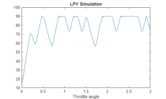
Generate open-loop response to an input along a parameter trajectory.
For this model, specify implicitly as a function of time , input , and state . Here is the throttle angle (first state).
load ThrottleInputData.mat
t2 = linspace(t(1),t(end),2000);
u2 = interp1(t,u,t2);
p = @(t,x,u)x(1);
yLPV = lsim(sysp,u2,t2,x0,p);
Plot the response.
plot(t2,yLPV)
title('LPV Simulation')
xlabel('Throttle angle')
Nonlinear Simulation
Simulate the nonlinear Simulink® model.
open_system('throttleNLModel')
ysl = sim('throttleNLModel');
ysl = interp1(ysl.ScopeData(:,1),ysl.ScopeData(:,2),t);
Compare the simulation results for the LPV and nonlinear models.
figure(1)
clf
plot(t,ysl,t2,yLPV)
legend('Simulink model','LPV model','location','Best')
title('Comparison of LPV and Nonlinear Simulations')
xlabel('Throttle angle')

The LPV model simulates the nonlinear response well because the model uses the actual trajectory for scheduling.
Close the model.
bdclose('throttleNLModel')Data Function
type throttleLPV.mfunction [A,B,C,D,E,dx0,x0,u0,y0,Delays] = throttleLPV(x1,c,k,b,K) % LPV representation of engine throttle dynamics. % Ref: https://www.mathworks.com/help/sldo/ug/estimate-model-parameter-values-gui.html % x1: scheduling parameter (throttle angle; first state of the model) % c,k,b,K: physical parameters A = [0 1; -k -c]; B = [0; b]; C = [1 0]; D = 0; E = []; Delays = []; x0 = []; u0 = []; y0 = []; % Nonlinear displacement value NLx = max(90,x1(1))-90+min(x1(1),15)-15; % Capture the nonlinear contribution as a state-derivative offset dx0 = [0;-K*NLx];
See Also
lpvss | sample | step | RespConfig