Rigid Assembly of Model Components
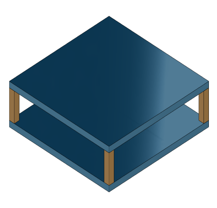
This example shows how to specify rigid physical coupling between the components of a structural model. Consider a structure that consists of two square plates connected with pillars at each vertex as depicted in the figure below. The lower plate is connected rigidly to the ground while the pillars are connected rigidly to each vertex of the square plates.
For more information on sparse models, see Sparse Model Basics.
platePillarModel.mat contains the sparse matrices for pillar and plate model. Load the finite element model matrices contained in platePillarModel.mat and create the sparse second-order state-space model representing the above system.
load('platePillarModel.mat')
Plate1 = mechss(M1,[],K1,B1,F1,'Name','Plate1');
Plate2 = mechss(M2,[],K2,B2,F2,'Name','Plate2');
Now, load the interfaced DOF index data from dofData.mat and use addInterface to create the coupling interfaces for connections between the two plates and the four pillars. dofs is a 6x7 cell array where the first two rows contain DOF index data for the first and second plate while the remaining four rows contain index data for the four pillars.
load('dofData.mat','dofs')
Define the interface for plates to pillars.
for ct=1:4
    Plate1 = addInterface(Plate1,"Pillar"+ct,dofs{1,2+ct});
    Plate2 = addInterface(Plate2,"Pillar"+ct,dofs{2,2+ct});
end
Define interface for pillars to plates.
P = cell(4,1);
for ct=1:4
    P{ct} = mechss(Mp,[],Kp,Bp,Fp,'Name',"Pillar"+ct);
    P{ct} = addInterface(P{ct},"TopMount",dofs{2+ct,1});
    P{ct} = addInterface(P{ct},"BottomMount",dofs{2+ct,2});
end
Define interface for Plate2 to ground.
Plate2 = addInterface(Plate2,"Ground",dofs{2,7});The resultant model sys has 5820 degrees of freedom, one input and one output. Use showStateInfo to examine the components of the mechss model object.
sys = append(Plate1,Plate2,P{:})Sparse continuous-time second-order model with 204 outputs, 204 inputs, and 5820 degrees of freedom. Model Properties Use "spy" and "showStateInfo" to inspect model structure. Type "help mechssOptions" for available solver options for this model.
showStateInfo(sys)
The state groups are:

    Type        Name      Size
  ----------------------------
  Component    Plate1     2646
  Component    Plate2     2646
  Component    Pillar1     132
  Component    Pillar2     132
  Component    Pillar3     132
  Component    Pillar4     132
The named components are listed in the output with their respective sizes.
Now, specify rigid couplings between the plates and the pillars.
sysCon = sys;
for ct=1:4
    sysCon = assemble(sysCon,"Plate1:Pillar"+ct,"Pillar"+ct+":TopMount"');
    sysCon = assemble(sysCon,"Plate2:Pillar"+ct,"Pillar"+ct+":BottomMount");
end
Specify rigid connection between the bottom plate and the ground.
sysCon = assemble(sysCon,"Plate2:Ground","Ground")
Sparse continuous-time second-order model with 6 outputs, 6 inputs, and 5922 degrees of freedom.
Model Properties

Use "spy" and "showStateInfo" to inspect model structure.
Type "help mechssOptions" for available solver options for this model.
Notice that the model now contains 5922 degrees of freedom. The extra DOFs are a result of the specific rigid interfaces.
assemble uses 'dual assembly' formulation to connect the components. In the concept of dual assembly, the global set of degrees of freedom (DoFs) is retained and the physical coupling is expressed as consistency and equilibrium constraints at the interface. For rigid connections, these constraints are of the form:
where is the vector of internal forces at the interface, and the matrix is permutable to . For a pair of matching DOFs with indices , where selects a DOF in the first component while selects the matching DOF in the second component, enforces consistency of displacements:
while enforces equilibrium of the internal forces at the interface:
.
Combining these constrains with the uncoupled equations leads to the following dual assembly model for the coupled system:
Use showStateInfo to confirm the physical connections.
showStateInfo(sysCon)
The state groups are:

    Type                      Name                   Size
  -------------------------------------------------------
  Component                  Plate1                  2646
  Component                  Plate2                  2646
  Component                 Pillar1                   132
  Component                 Pillar2                   132
  Component                 Pillar3                   132
  Component                 Pillar4                   132
  Interface     Plate1:Pillar1-Pillar1:TopMount        12
  Interface    Plate2:Pillar1-Pillar1:BottomMount      12
  Interface     Plate1:Pillar2-Pillar2:TopMount        12
  Interface    Plate2:Pillar2-Pillar2:BottomMount      12
  Interface     Plate1:Pillar3-Pillar3:TopMount        12
  Interface    Plate2:Pillar3-Pillar3:BottomMount      12
  Interface     Plate1:Pillar4-Pillar4:TopMount        12
  Interface    Plate2:Pillar4-Pillar4:BottomMount      12
  Interface           Plate2:Ground-Ground              6
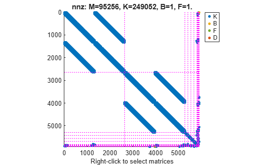
You can use spy to visualize the sparse matrices in the final model. Choose between the matrices to be displayed using the display menu that can be accessed by right-clicking on the plot.
spy(sysCon)
Acknowledgements
The data set for this example was provided by Victor Dolk from ASML.
See Also
addInterface | assemble | xsort | showStateInfo | spy | mechss