Multivariate Tensor Product Splines
Introduction to Multivariate Tensor Product Splines
The toolbox provides (polynomial) spline functions in any number of variables, as tensor products of univariate splines. These multivariate splines come in both standard forms, the B-form and the ppform, and their construction and use parallels entirely that of the univariate splines discussed in previous sections, Constructing and Working with ppform Splines and Constructing and Working with B-form Splines. The same commands are used for their construction and use.
For simplicity, the following discussion deals just with bivariate splines.
B-form of Tensor Product Splines
The tensor-product idea is very simple. If f is a function of x, and g is a function of y, then their tensor-product p(x,y) := f(x)g(y) is a function of x and y, i.e., a bivariate function. More generally, with s = (s1,...,sm+h) and t = (t1,...,tn+k) knot sequences and aij (i = 1,...,m; j = 1,...n) a corresponding coefficient array, you obtain a bivariate spline as
The B-form of this spline comprises the cell array {s,t} of its knot sequences, the coefficient array a, the numbers vector [m,n], and the orders vector [h,k]. The command
sp = spmak({s,t},a);
constructs this form. Further, fnplt, fnval,
fnder, fndir, fnrfn, and
fn2fm can be used to plot, evaluate, differentiate and integrate,
refine, and convert this form.
Construction With Gridded Data
You are most likely to construct such a form by looking for an interpolant or
approximant to gridded data. For example, if you know the values z(i,j)=g(x(i),y(j)),i=1:m,
j=1:n, of some function g at all the points in a
rectangular grid, then, assuming that the strictly increasing sequence x
satisfies the Schoenberg-Whitney conditions with respect to the above knot
sequence s, and that the strictly increasing sequence
y satisfies the Schoenberg-Whitney conditions with respect to the
above knot sequence t, the command
sp=spapi({s,t},[h,k],{x,y},z);constructs the unique bivariate spline of the above form that matches the given
values. The command fnplt(sp) gives you a quick plot of this
interpolant. The command pp = fn2fm(sp,'pp') gives you the ppform of
this spline, which is probably what you want when you want to evaluate the spline at a
fine grid((xx(i),yy(j)) for i=1:M, j=1:N), by the
command:
values = fnval(pp,{xx,yy});
ppform of Tensor Product Splines
The ppform of such a bivariate spline comprises, analogously, a cell array of break
sequences, a multidimensional coefficient array, a vector of number pieces, and a vector
of polynomial orders. Fortunately, the toolbox is set up in such a way that there is
usually no reason for you to concern yourself with these details of either form. You use
interpolation, approximation, or smoothing to construct splines, and then use the
fn... commands to make use of them.
Example: The Mobius Band
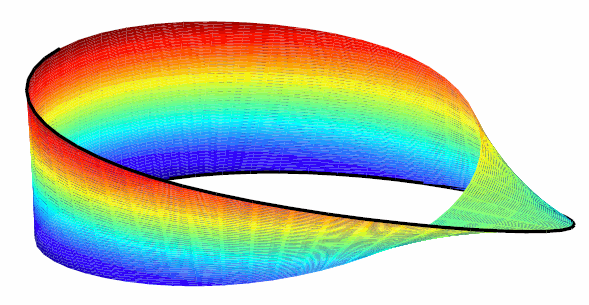
Here is an example of a surface constructed as a 3-D-valued bivariate spline. The surface is the famous Möbius band, obtainable by taking a longish strip of paper and gluing its narrow ends together, but with a twist. The figure is obtained by the following commands:
x = 0:1; y = 0:4; h = 1/4; o2 = 1/sqrt(2); s = 2; ss = 4;
v(3,:,:) = h*[0, -1, -o2, 0, o2, 1, 0;0, 1, o2, 0, -o2, -1, 0];
v(2,:,:) = [ss, 0, s-h*o2, 0, -s-h*o2, 0, ss;...
            ss, 0, s+h*o2, 0,-s+h*o2, 0, ss];
v(1,:,:) = s*[0, 1, 0, -1+h, 0, 1, 0; 0, 1, 0, -1-h, 0, 1, 0];
cs = csape({x,y},v,{'variational','clamped'});
fnplt(cs), axis([-2 2 -2.5 2.5 -.5 .5]), shading interp
axis off, hold on
values = squeeze(fnval(cs,{1,linspace(y(1),y(end),51)}));
plot3(values(1,:), values(2,:), values(3,:),'k','linew',2)
view(-149,28), hold off
A Möbius Band Made by Vector-Valued Bivariate Spline Interpolation
