Neural Network for Digital Predistortion Design - Online Training

This example uses:

This example shows how to create an online training neural network digital predistortion (DPD) system to offset the effects of nonlinearities in a power amplifier (PA) using a custom training loop. The custom training loop contains

OFDM signal generation,
NN-DPD processing,
PA measurements using a VST,
Performance metric calculation, and
Weight update control logic.

Introduction

Nonlinear behavior in PAs result in severe signal distortions and cause challenges for error-free reception of the high-frequency and high-bandwidth signals commonly transmitted in 5G NR [1]. DPD of the transmitted signal is a technique used to compensate for PA nonlinearities that distort the signal. The Neural Network for Digital Predistortion Design - Offline Training (Communications Toolbox) example focuses on the offline training of a neural network DPD. In the offline training system, once the training is done, the NN-DPD weights are kept constant. If the PA characteristics change, the system performance may suffer.

In an online training system, the NN-DPD weights can be updated based on predetermined performance metrics. This diagram shows the online training system. There are two NN-DPDs in this system. The NN-DPD-Forward is used in the signal path to apply digital predistortion to the signals. The input of this NN-DPD is the oversampled communication signal and its output is connected to the PA. The NN-DPD-Train is used to update the NN-DPD weights and biases. Its input signal is the PA output and the training target is the PA input. As a result, the NN-DPD is trained as the inverse of the PA.

The following is the flow diagram of the online training system. When the system first starts running, NN-DPD weights are initialized randomly. As a result, the output of the NN-DPD is not a valid signal. Bypass the NN-DPD-Forward until the NN-DPD-Train trains to an initial valid state. Once the initialization is done, pass the signals through the NN-DPD-Forward. Calculate normalized mean square error (NMSE) using the signal at the input of the NN-DPD-Forward and at the output of the PA. If the NMSE is higher than a threshold, then update the NN-DPD-Train weights and biases using the current frame's I/Q samples. Once the update finishes, copy the weights and biases to the NN-DPD-Forward. If the NMSE is lower than the threshold, then do not update the NN-DPD-Train. The NN-DPD updates are done asynchronously.

Generate Oversampled OFDM Signals

Generate OFDM-based signals to excite the PA. This example uses a 5G-like OFDM waveform. Set the bandwidth of the signal to 100 MHz. Choosing a larger bandwidth signal causes the PA to introduce more nonlinear distortion and yields greater benefit from the addition of the DPD. Generate six OFDM symbols, where each subcarrier carries a 16-QAM symbol, using the ofdmmod (Communications Toolbox) and qammod (Communications Toolbox) function. Save the 16-QAM symbols as a reference to calculate the EVM performance. To capture effects of higher order nonlinearities, the example oversamples the PA input by a factor of 5.

bw = 100e6;       % Hz
symPerFrame = 6;  % OFDM symbols per frame
M = 16;           % Each OFDM subcarrier contains a 16-QAM symbol
osf = 5;          % oversampling factor for PA input

% OFDM parameters
ofdmParams = helperOFDMParameters(bw,osf);
numDataCarriers = (ofdmParams.fftLength - ofdmParams.NumGuardBandCarrier - 1);
nullIdx = [1:ofdmParams.NumGuardBandCarrier/2+1 ...
  ofdmParams.fftLength-ofdmParams.NumGuardBandCarrier/2+1:ofdmParams.fftLength]';
Fs = ofdmParams.SampleRate;

% Random data
x = randi([0 M-1],numDataCarriers,symPerFrame);

% OFDM with 16-QAM in data subcarriers
qamRefSym = qammod(x, M);
dpdInput = single(ofdmmod(qamRefSym/osf,ofdmParams.fftLength,ofdmParams.cpLength,...
  nullIdx,OversamplingFactor=osf));

NN-DPD

NN-DPD has three fully connected hidden layers followed by a fully connected output layer. Memory length and degree of nonlinearity determine the input length, as described in the Power Amplifier Characterization (Communications Toolbox) example. Set the memory depth to 5 and degree of nonlinearity to 5. Custom training loops require dlnetwork objects. Create a dlnetwork for the NN-DPD-Forward and another for the NN-DPD-Train.

memDepth = 5;            % Memory depth of the DPD (or PA model)
nonlinearDegree = 5;     % Nonlinear polynomial degree
inputLayerDim = 2*memDepth+(nonlinearDegree-1)*memDepth;
numNeuronsPerLayer = 40;

layers = [...
  featureInputLayer(inputLayerDim,'Name','input')

  fullyConnectedLayer(numNeuronsPerLayer,'Name','linear1')
  leakyReluLayer(0.01,'Name','leakyRelu1')

  fullyConnectedLayer(numNeuronsPerLayer,'Name','linear2')
  leakyReluLayer(0.01,'Name','leakyRelu2')

  fullyConnectedLayer(numNeuronsPerLayer,'Name','linear3')
  leakyReluLayer(0.01,'Name','leakyRelu3')

  fullyConnectedLayer(2,'Name','linearOutput')];

netTrain = dlnetwork(layers);
netForward = dlnetwork(layers);

The input to the NN-DPD is preprocessed as described in Neural Network for Digital Predistortion Design - Offline Training (Communications Toolbox) example. Create input preprocessing objects for both NN-DPDs.

inputProcTrain = helperNNDPDInputLayer(memDepth,nonlinearDegree);
inputProcForward = helperNNDPDInputLayer(memDepth,nonlinearDegree);

Since the dlnetTrain and dlnetForward are not trained yet, bypass the NN-DPD.

dpdOutput = dpdInput;

Power Amplifier

Choose the data source for the system. This example uses an NXP Airfast LDMOS Doherty PA, which is connected to a local NI VST, as described in the Power Amplifier Characterization (Communications Toolbox) example. If you do not have access to a PA, run the example with saved data or simulated PA. Simulated PA uses a neural network PA model, which is trained using data captured from the PA using an NI VST.

dataSource = "Simulated PA";

Pass the signal through the PA and measure the output signal using an NI VST. Lower target input power values may cause less distortion.

if strcmp(dataSource,"NI VST")
  targetInputPower = 5; % dBm
  VST = helperVSTDriver('VST_01');
  VST.DUTExpectedGain     = 29;                % dB
  VST.ExternalAttenuation = 30;                % dB
  VST.DUTTargetInputPower = targetInputPower;  % dBm
  VST.CenterFrequency     = 3.7e9;             % Hz

  % Send the signals to the PA and collect the outputs
  paOutput = helperNNDPDPAMeasure(dpdOutput,Fs,VST);
elseif strcmp(dataSource,"Simulated PA")
  load paModelNN.mat netPA memDepthPA nonlinearDegreePA scalingFactorPA
  inputProcPA = helperNNDPDInputLayer(memDepthPA,nonlinearDegreePA);
  inputProcPAMP = helperNNDPDInputLayer(memDepthPA,nonlinearDegreePA);

  X = process(inputProcPA,dpdOutput*scalingFactorPA);
  Y = predict(netPA,X);
  paOutput = complex(Y(:,1), Y(:,2));
  paOutput = paOutput / scalingFactorPA;
else
  load nndpdInitTrainingData paOutput dpdInput
  dpdOutput = dpdInput;
end

Custom Training Loop

Create a custom training loop to train the NN-DPD-Train to an initial valid state. Custom training loop has these parts:

for-loop over epochs
mini-batch queue to handle mini-batch selection
while-loop over mini-batches
model gradients, state, and loss evaluation
network parameter update
learning rate control
training information logging

Run the epoch loop for maxNumEpochs. Set minibatch size to miniBatchSize. Larger values of mini-batch size yields to faster training but may require larger learning rate. Set the initial learning rate to initLearnRate and update the learning rate each learnRateDropPeriod number of epochs by a factor of learnRateDropFactor. Also, set a minimum learning rate value to avoid training to practically stop.

% Training options
maxNumEpochs = 40;
miniBatchSize = 4096;        % I/Q samples
initLearnRate = 2e-2;
minLearnRate = 1e-5;
learnRateDropPeriod = 20;    % Epochs
learnRateDropFactor = 0.2;

iterationsPerBatch = floor(length(dpdOutput)/miniBatchSize);

References [2] and [3] describe the benefit of normalizing the input signal to avoid the gradient explosion problem and ensure that the neural network converges to a better solution. Normalization requires obtaining a unity standard deviation and zero mean. For this example, the communication signals already have zero mean, so normalize only the standard deviation. Later, you need to denormalize the NN-DPD output values by using the same scaling factor.

scalingFactor = 1/std(dpdOutput);

Preprocess input and ouput signals.

trainInputMtx = process(inputProcTrain, ...
  paOutput*scalingFactor);

trainOutputBatchC = dpdOutput*scalingFactor;
trainOutputBatchR = [real(trainOutputBatchC) imag(trainOutputBatchC)];

Create two arrayDatastore objects and combine them to represent the input and target relationship. The dsInput stores the input signal, X, and the dsOutput stores the target signals, T, for the NN-DPD-Train.

dsInput = arrayDatastore(trainInputMtx, ...
  IterationDimension=1,ReadSize=miniBatchSize);
dsOutput = arrayDatastore(trainOutputBatchR, ...
  IterationDimension=1,ReadSize=miniBatchSize);
cds = combine(dsInput,dsOutput);

Create a minibatchqueue object to automate the mini batch fetching. First dimension is time dimension and is labeled as batch, B, to instruct the network to interpret every individual timestep as an independent observation. Second dimension is the features dimension and is labeled as C. Since the data size is small, the training loop runs faster on CPU. Set OutputEnvironment for both input and target data as 'cpu'.

mbq = minibatchqueue(cds,...
  MiniBatchSize=miniBatchSize,...
  PartialMiniBatch="discard",...
  MiniBatchFormat=["BC","BC"],...
  OutputEnvironment={'cpu','cpu'});

For each iteration, fetch input and target data from the mini-batch queue. Evaluate the model gradients, state, and loss using dlfeval function with custom modelLoss function. Then update the network parameters using the Adam optimizer function, adamupdate. For more information on custom training loops, see Define Custom Training Loops, Loss Functions, and Networks.

When running the example, you have the option of using a pretrained network by setting the trainNow variable to false. Training is desirable to match the network to your simulation configuration. If using a different PA, signal bandwidth, or target input power level, retrain the network. Training the neural network on an Intel® Xeon® W-2133 CPU @ 3.60GHz takes less than 3 minutes.

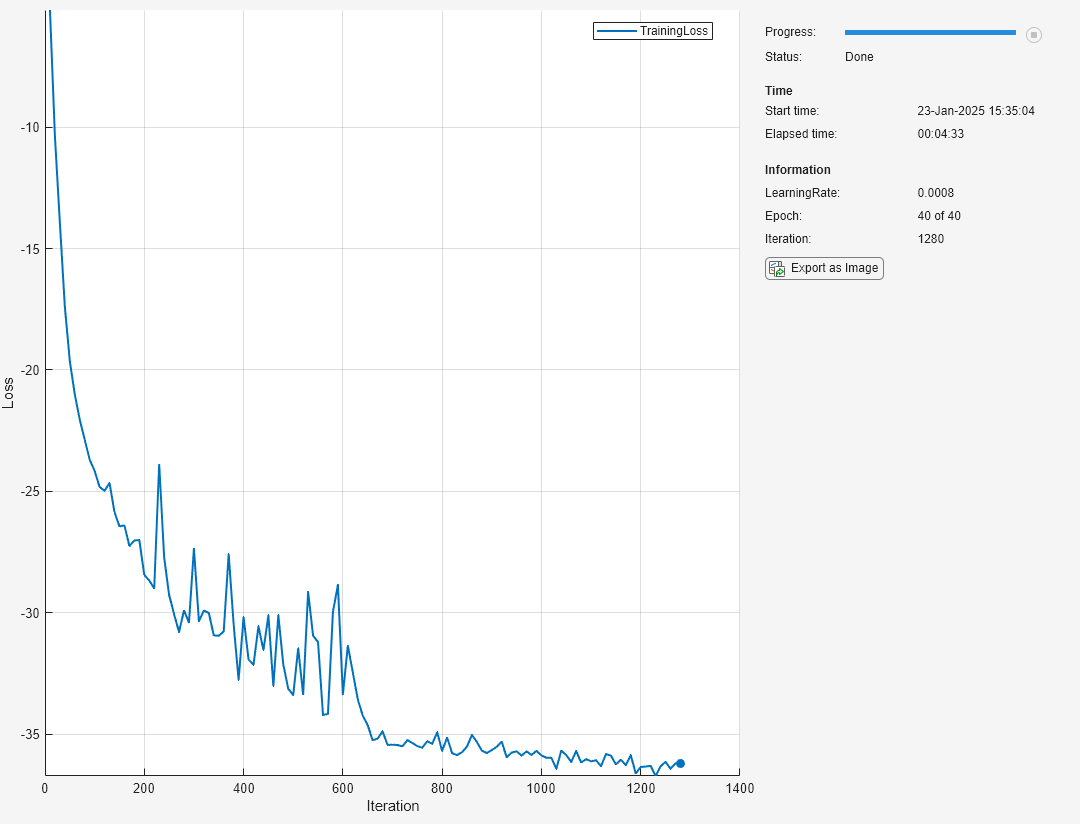
trainNow = true;
if trainNow
  % Initialize training progress monitor
  monitor = trainingProgressMonitor;
  monitor.Info = ["LearningRate","Epoch","Iteration"];
  monitor.Metrics = "TrainingLoss";
  monitor.XLabel = "Iteration";
  groupSubPlot(monitor,"Loss","TrainingLoss");
  monitor.Status = "Running";
  plotUpdateFrequency = 10;

  % Initialize training loop
  averageGrad = [];
  averageSqGrad = [];
  learnRate = initLearnRate;
  iteration = 1;

  for epoch = 1:maxNumEpochs
    shuffle(mbq)

    % Update learning rate
    if mod(epoch,learnRateDropPeriod) == 0
      learnRate = learnRate * learnRateDropFactor;
    end

    % Loop over mini-batches
    while hasdata(mbq) && ~monitor.Stop
      % Process one mini-batch of data
      [X,T] = next(mbq);

      % Evaluate model gradients and loss
      [lossTrain,gradients] = dlfeval(@modelLoss,netTrain,X,T);

      % Update network parameters
      [netTrain,averageGrad,averageSqGrad] = ...
        adamupdate(netTrain,gradients,averageGrad,averageSqGrad, ...
        iteration,learnRate);

      if mod(iteration,plotUpdateFrequency) == 0
        updateInfo(monitor, ...
          LearningRate=learnRate, ...
          Epoch=string(epoch) + " of " + string(maxNumEpochs), ...
          Iteration=string(iteration));
        recordMetrics(monitor,iteration, ...
          TrainingLoss=10*log10(lossTrain));
      end

      iteration = iteration + 1;
    end
    if monitor.Stop
      break
    end
    monitor.Progress = 100*epoch/maxNumEpochs;
  end
  if monitor.Stop
    monitor.Status = "User terminated";
  else
    monitor.Status = "Done";
  end
else
  load offlineTrainedNNDPDR2023a netTrain learnRate learnRateDropFactor ...
    learnRateDropPeriod maxNumEpochs miniBatchSize scalingFactor ...
    symPerFrame monitor averageGrad averageSqGrad
end

Online Training with HIL

Convert the previous custom training loop to an online training loop with hardware-in-the-loop processing, where the hardware is the PA. Perform following modifications:

Add OFDM signal generation,
Copy NN-DPD-Train learnables to NN-DPD-Forward and apply predistortion using the forward function,
Send the predistorted signal to PA and measure the output,
Compute performance metric, which is NMSE,
If the performance metric is out of spec, then update the NN-DPD-Train learnables with the custom loop shown in the Custom Training Loop section without epoch processing,
Add memory polynomial based DPD for comparison using comm.DPDCoefficientEstimator (Communications Toolbox) and comm.DPD (Communications Toolbox) System objects.

Run the online training loop for maxNumFrames frames. Set the target NMSE to targetNMSE dB with a margin of targetNMSEMargin dB. The margin creates a hysteresis where the training is stopped if NMSE is less than targetNMSE-targetNMSEMargin and started if NMSE is greater than targetNMSE+targetNMSEMargin.

maxNumFrames = 200;           % Frames
if strcmp(dataSource,"NI VST") || strcmp(dataSource,"Saved data")
  targetNMSE = -33.5;         % dB
else
  targetNMSE = -30.0;         % dB
end
targetNMSEMargin = 0.5;       % dB

Initialize NN-DPD-Forward.

netForward.Learnables = netTrain.Learnables;

Configure the learning rate schedule. Start with learnRate and drop by a factor of learnRateDropFactor every learnRateDropPeriod frames.

learnRateDropPeriod = 100;
learnRateDropFactor = 0.5;
learnRate = 0.0001;

Initialize memory polynomial based DPD.

polynomialType = "Memory polynomial"; 
estimator = comm.DPDCoefficientEstimator( ...
  DesiredAmplitudeGaindB=0, ...
  PolynomialType=polynomialType, ...
  Degree=nonlinearDegree, ...
  MemoryDepth=memDepth, ...
  Algorithm='Least squares');
coef = estimator(dpdOutput,paOutput);

Warning: Rank deficient, rank = 9, tol =  1.112654e-03.

dpdMem = comm.DPD(PolynomialType=polynomialType, ...
  Coefficients=coef);

If trainNow is true and dataSource is not "Saved data", run the online training loop.

trainNow = false;
if trainNow && ~strcmp(dataSource,"Saved data")
  % Turn off warning for the loop
  warnState = warning('off','MATLAB:rankDeficientMatrix');
  clup = onCleanup(@()warning(warnState));

  % Initialize training progress monitor
  monitor = trainingProgressMonitor;
  monitor.Info = ["LearningRate","Frames","Iteration"];
  monitor.Metrics = ["TrainingLoss","NMSE","NMSE_MP"];
  monitor.XLabel = "Iteration";
  groupSubPlot(monitor,"Loss","TrainingLoss");
  groupSubPlot(monitor,"System Metric",{"NMSE","NMSE_MP"});
  monitor.Status = "Running";
  plotUpdateFrequency = 10;

  % Reset input preprocessing objects
  reset(inputProcTrain);
  reset(inputProcForward);

  numFrames = 1;
  iteration = 1;
  maxNumIterations = maxNumFrames*iterationsPerBatch;
  updateFrameCounter = 1;
  while numFrames < maxNumFrames && ~monitor.Stop
    % Generate OFDM I/Q samples
    x = randi([0 M-1], numDataCarriers, symPerFrame);
    qamRefSym = qammod(x, M);
    dpdInput = single(ofdmmod(qamRefSym/osf,ofdmParams.fftLength,ofdmParams.cpLength,...
      nullIdx,OversamplingFactor=osf));

    dpdInputMtx = process(inputProcForward,dpdInput*scalingFactor);

    % Send one frame of data to NN-DPD
    X = dlarray(dpdInputMtx, "BC"); % B: batch size; C: number of features (dimension in input layer of the neural network)
    [Y,~] = forward(netForward,X);
    dpdOutput = (extractdata(Y))';
    dpdOutput = complex(dpdOutput(:,1), dpdOutput(:,2));
    % Normalize output signal
    dpdOutput = dpdOutput / scalingFactor;

    % Send one frame of data to memory polynomial DPD
    dpdOutputMP = dpdMem(dpdInput);
    
    % Send DPD outputs through PA
    if strcmp(dataSource,"NI VST")
      paOutput = helperNNDPDPAMeasure(dpdOutput,Fs,VST);
      paOutputMP = helperNNDPDPAMeasure(dpdOutputMP,Fs,VST);
    else % "Simulated PA"
      paInputMtx = process(inputProcPA,dpdOutput*scalingFactorPA);
      paOutput = predict(netPA,paInputMtx);
      paOutput = complex(paOutput(:,1), paOutput(:,2));
      paOutput = paOutput / scalingFactorPA;

      paInputMtxMP = process(inputProcPAMP,dpdOutputMP*scalingFactorPA);
      paOutputMP = predict(netPA,paInputMtxMP);
      paOutputMP = complex(paOutputMP(:,1), paOutputMP(:,2));
      paOutputMP = paOutputMP / scalingFactorPA;
    end

    % Compute NMSE
    nmseNN = localNMSE(dpdInput, paOutput);
    nmseMP = localNMSE(dpdInput, paOutputMP);

    % Check if NMSE is too large
    if updateNNDPDWeights(nmseNN,targetNMSE,targetNMSEMargin)
      % Need to update the weights/biases of the neural network DPD

      % Preprocess input and output of the NN
      trainInputMtx = process(inputProcForward, ...
        paOutput*scalingFactor);
      trainOutputBatchC = dpdOutput*scalingFactor;
      trainOutputBatchR = [real(trainOutputBatchC) imag(trainOutputBatchC)];

      % Create combined data store
      dsInput = arrayDatastore(trainInputMtx, ...
        IterationDimension=1,ReadSize=miniBatchSize);
      dsOutput = arrayDatastore(trainOutputBatchR, ...
        IterationDimension=1,ReadSize=miniBatchSize);
      cds = combine(dsInput,dsOutput);

      % Create mini-batch queue for the combined data store
      mbq = minibatchqueue(cds,...
        MiniBatchSize=miniBatchSize,...
        PartialMiniBatch="discard",...
        MiniBatchFormat=["BC","BC"],...
        OutputEnvironment={'cpu','cpu'});

      % Update learning rate based on the schedule
      if mod(updateFrameCounter, learnRateDropPeriod) == 0 ...
          && learnRate > minLearnRate
        learnRate = learnRate*learnRateDropFactor;
      end

      % Loop over mini-batches
      while hasdata(mbq) && ~monitor.Stop
        % Process one mini-batch of data
        [X,T] = next(mbq);

        % Evaluate the model gradients, state, and loss
        [lossTrain,gradients] = dlfeval(@modelLoss,netTrain,X,T);

        % Update the network parameters
        [netTrain,averageGrad,averageSqGrad] = ...
          adamupdate(netTrain,gradients,averageGrad,averageSqGrad, ...
          iteration,learnRate);

        iteration = iteration + 1;
        if mod(iteration,plotUpdateFrequency) == 0 && hasdata(mbq)
          % Every plotUpdateFrequency iterations, update training monitor
          updateInfo(monitor, ...
            LearningRate=learnRate, ...
            Frames=string(numFrames) + " of " + string(maxNumFrames), ...
            Iteration=string(iteration) + " of " + string(maxNumIterations));

          recordMetrics(monitor,iteration, ...
            TrainingLoss=10*log10(lossTrain));

          monitor.Progress = 100*iteration/maxNumIterations;
        end
      end

      netForward.Learnables = netTrain.Learnables;

      % Update memory polynomial DPD
      coef = estimator(dpdOutputMP,paOutputMP);
      dpdMem.Coefficients = coef;

      updateFrameCounter = updateFrameCounter + 1;
    else
      iteration = iteration + iterationsPerBatch;
    end

    updateInfo(monitor, ...
      LearningRate=learnRate, ...
      Frames=string(numFrames)+" of "+string(maxNumFrames), ...
      Iteration=string(iteration)+" of "+string(maxNumIterations));

    recordMetrics(monitor, iteration, ...
      TrainingLoss=10*log10(lossTrain), ...
      NMSE=nmseNN, ...
      NMSE_MP=nmseMP);

    monitor.Progress = 100*numFrames/maxNumFrames;
    numFrames = numFrames + 1;
  end
  if monitor.Stop
    monitor.Status = "User terminated";
  else
    monitor.Status = "Done";
  end
  if strcmp(dataSource,"NI VST")
    release(VST)
  end
  clear clup
else
  % Load saved results
    load onlineTrainedNNDPDR2023a netTrain learnRate learnRateDropFactor ...
      learnRateDropPeriod maxNumEpochs miniBatchSize scalingFactor ...
      symPerFrame monitor averageGrad averageSqGrad
    load onlineStartNNDPDPAData dpdOutput dpdOutputMP paOutput paOutputMP qamRefSym nmseNN nmseMP
end

The online training progress shows that the NN-DPD can achieve about 7 dB better average NMSE as compared to the memory polynomial DPD. Horizontal regions in the Loss plot show the regions where the NN-DPD weights were kept constant.

Compare Neural Network and Memory Polynomial DPDs

Compare the PA output spectrums for the NN-DPD and memory polynomial DPD. Plot the power spectrum for PA output with NN-DPD and memory polynomial DPD. The NN-DPD achieves more sideband suppression as compared to the memory polynomial DPD.

pspectrum(paOutput,Fs,'MinThreshold',-120)
hold on
pspectrum(paOutputMP,Fs,'MinThreshold',-120)
hold off
legend("NN-DPD","Memory Polynomial")
title("Power Spectrum of PA Output")

Figure contains an axes object. The axes object with title Power Spectrum of PA Output, xlabel Frequency (MHz), ylabel Power Spectrum (dB) contains 2 objects of type line. These objects represent NN-DPD, Memory Polynomial.

Calculate ACPR and EVM values and show the results. The NN-DPD achieves about 6 dB better ACPR and NMSE as compared to the memory polynomial DPD. The percent EVM for the NN-DPD is about half of the memory polynomial DPD.

acprNNDPD = localACPR(paOutput,Fs,bw);
acprMPDPD = localACPR(paOutputMP,Fs,bw);
evmNNDPD = localEVM(paOutput,qamRefSym(:),ofdmParams);
evmMPDPD = localEVM(paOutputMP,qamRefSym(:),ofdmParams);

% Create a table to display results
evm = [evmMPDPD;evmNNDPD];
acpr = [acprMPDPD;acprNNDPD];
nmse = [nmseMP; nmseNN];
disp(table(acpr,nmse,evm, ...
  'VariableNames', ...
  {'ACPR_dB','NMSE_dB','EVM_percent'}, ...
  'RowNames', ...
  {'Memory Polynomial DPD','Neural Network DPD'}))

                             ACPR_dB    NMSE_dB    EVM_percent
                             _______    _______    ___________

    Memory Polynomial DPD    -33.695    -27.373        3.07   
    Neural Network DPD       -39.237    -33.276      1.5996

Appendix: Neural Network Model of PA

Train a neural network PA model (NN-PA) to use for online simulations. NN-PA has three fully connected hidden layers followed by a fully connected output layer. Set the memory depth to 5 and degree of nonlinearity to 5.

memDepthPA = 5;            % Memory depth of the DPD (or PA model)
nonlinearDegreePA = 5;     % Nonlinear polynomial degree
inputLayerDim = 2*memDepthPA+(nonlinearDegreePA-1)*memDepthPA;
numNeuronsPerLayer = 40;

layers = [...
  featureInputLayer(inputLayerDim,'Name','input')

  fullyConnectedLayer(numNeuronsPerLayer,'Name','linear1')
  leakyReluLayer(0.01,'Name','leakyRelu1')

  fullyConnectedLayer(numNeuronsPerLayer,'Name','linear2')
  leakyReluLayer(0.01,'Name','leakyRelu2')

  fullyConnectedLayer(numNeuronsPerLayer,'Name','linear3')
  leakyReluLayer(0.01,'Name','leakyRelu3')

  fullyConnectedLayer(2,'Name','linearOutput')
  
  regressionLayer("Name","regressionoutput")
  ];

Create input preprocessing objects for both NN-DPDs.

inputProcPA = helperNNDPDInputLayer(memDepthPA,nonlinearDegreePA);

Load the training data collected at the input and output of the PA.

load nndpdInitTrainingData paOutput dpdInput Fs
paInput = dpdInput;

Preprocess the input and output signals.

scalingFactorPA = 1/std(paInput);

trainInputMtx = process(inputProcPA, ...
  paInput*scalingFactorPA);

trainOutputBatchC = paOutput*scalingFactorPA;
trainOutputBatchR = [real(trainOutputBatchC) imag(trainOutputBatchC)];

Train the NN-PA

options = trainingOptions('adam', ...
    MaxEpochs=1000, ...
    MiniBatchSize=4096*2, ...
    InitialLearnRate=2e-2, ...
    LearnRateDropFactor=0.5, ...
    LearnRateDropPeriod=50, ...
    LearnRateSchedule='piecewise', ...
    Shuffle='every-epoch', ...
    ExecutionEnvironment='cpu', ...
    Plots='training-progress', ...
    Verbose=false);

trainNow = false;
if trainNow
  [netPA,trainInfo] = trainNetwork(trainInputMtx,trainOutputBatchR,layers,options); %#ok<UNRCH> 
  lg = layerGraph(netPA);
  lg = lg.removeLayers('regressionoutput');
  dlnetPA = dlnetwork(lg);
else
  load paModelNN netPA dlnetPA memDepthPA nonlinearDegreePA
end

Compare Neural Network and Memory Polynomial PAs

Compare the PA output spectrums for the NN-PA and memory polynomial PA. Since a DPD tries to model the inverse of a PA, use comm.DPD and comm.DPDCoefficientEstimator to model a memory polynomial PA by reversing the paOutput and paInput inputs to the estimator.

estimator = comm.DPDCoefficientEstimator( ...
  DesiredAmplitudeGaindB=0, ...
  PolynomialType=polynomialType, ...
  Degree=nonlinearDegreePA, ...
  MemoryDepth=memDepthPA, ...
  Algorithm='Least squares');
coef = estimator(paOutput,paInput);

Warning: Rank deficient, rank = 9, tol =  1.107856e-03.

paMem = comm.DPD(PolynomialType=polynomialType, ...
  Coefficients=coef);
paOutputMP = paMem(paInput);

paInputMtx = process(inputProcPA,dpdInput*scalingFactorPA);
X = dlarray(paInputMtx, "BC");
[Y,~] = forward(dlnetPA,X);
paOutputNN = (extractdata(Y))';
paOutputNN = double(complex(paOutputNN(:,1), paOutputNN(:,2)));
% Normalize output signal
paOutputNN = paOutputNN / scalingFactorPA;

pspectrum(paOutput,Fs,'MinThreshold',-120)
hold on
pspectrum(paOutputMP,Fs,'MinThreshold',-120)
pspectrum(paOutputNN,Fs,'MinThreshold',-120)
hold off
legend("Original","Memory Polynomial","NN-PA")
title("Power Spectrum of PA Output")

Figure contains an axes object. The axes object with title Power Spectrum of PA Output, xlabel Frequency (MHz), ylabel Power Spectrum (dB) contains 3 objects of type line. These objects represent Original, Memory Polynomial, NN-PA.

Calculate ACPR, NMSE and EVM values and show the results. The NN-PA model better approximates the PA as compared to the memory polynomial model.

acprPA = localACPR(paOutput,Fs,bw);
acprMPPA = localACPR(paOutputMP,Fs,bw);
acprNNPA = localACPR(paOutputNN,Fs,bw);

[evmPA,rxQAMSymPA] = localEVM(paOutput,[],ofdmParams);
[evmMPPA,rxQAMSymMP] = localEVM(paOutputMP,[],ofdmParams);
[evmNNPA,rxQAMSymNN] = localEVM(paOutputNN,[],ofdmParams);

nmsePA = localNMSE(paOutput,paOutput);
nmseMPPA = localNMSE(paOutputMP,paOutput);
nmseNNPA = localNMSE(paOutputNN,paOutput);

% Create a table to display results
evm = [evmPA;evmMPPA;evmNNPA];
acpr = [acprPA;acprMPPA;acprNNPA];
nmse = [nmsePA;nmseMPPA;nmseNNPA];
disp(table(acpr,nmse,evm, ...
  'VariableNames', ...
  {'ACPR_dB','NMSE_dB','EVM_percent'}, ...
  'RowNames', ...
  {'Original','Memory Polynomial PA','Neural Network PA'}))

                            ACPR_dB    NMSE_dB    EVM_percent
                            _______    _______    ___________

    Original                -28.736       -Inf      6.7036   
    Memory Polynomial PA    -30.254    -27.166      5.9301   
    Neural Network PA       -28.874    -34.643      6.5409

References

[1] C. Tarver, L. Jiang, A. Sefidi and J. R. Cavallaro, "Neural Network DPD via Backpropagation through a Neural Network Model of the PA," 2019 53rd Asilomar Conference on Signals, Systems, and Computers, Pacific Grove, CA, USA, 2019, pp. 358-362, doi: 10.1109/IEEECONF44664.2019.9048910.

[2] J. Sun, J. Wang, L. Guo, J. Yang and G. Gui, "Adaptive Deep Learning Aided Digital Predistorter Considering Dynamic Envelope," IEEE Transactions on Vehicular Technology, vol. 69, no. 4, pp. 4487-4491, April 2020, doi: 10.1109/TVT.2020.2974506.

[3] J. Sun, W. Shi, Z. Yang, J. Yang and G. Gui, "Behavioral Modeling and Linearization of Wideband RF Power Amplifiers Using BiLSTM Networks for 5G Wireless Systems," in IEEE Transactions on Vehicular Technology, vol. 68, no. 11, pp. 10348-10356, Nov. 2019, doi: 10.1109/TVT.2019.2925562.

Appendix: Helper Functions

Signal Measurement and Input Processing

Performance Evaluation and Comparison

Local Functions

Normalized mean squared error (NMSE)

function nmseIndB = localNMSE(input,output)
%localNMSE Normalized mean squared error (NMSE)
%   E = localNMSE(X,Y) calculates the NMSE between X and Y.

nmse = sum(abs(input-output).^2) / sum(abs(input).^2);
nmseIndB = 10*log10(nmse);
end

Error vector magnitude (EVM)

function [rmsEVM,rxQAMSym] = localEVM(paOutput,qamRefSym,ofdmParams)
%localEVM Error vector magnitude (EVM)
%   [E,Y] = localEVM(X,REF,PARAMS) calculates EVM for signal, X, given the
%   reference signal, REF. X is OFDM modulated based on PARAMS.

% Downsample and demodulate
waveform = ofdmdemod(paOutput,ofdmParams.fftLength,ofdmParams.cpLength,...
    ofdmParams.cpLength,[1:ofdmParams.NumGuardBandCarrier/2+1 ...
     ofdmParams.fftLength-ofdmParams.NumGuardBandCarrier/2+1:ofdmParams.fftLength]',...
     OversamplingFactor=ofdmParams.OversamplingFactor);
rxQAMSym = waveform(:)*ofdmParams.OversamplingFactor;

if isempty(qamRefSym)
  M = 16;
  qamRefSym = qammod(qamdemod(rxQAMSym,M),M);
end

% Compute EVM
evm = comm.EVM;
rmsEVM = evm(qamRefSym,rxQAMSym);
end

Adjacent channel power ratio (ACPR)

function acpr = localACPR(paOutput,sr,bw)
%localACPR Adjacent channel power ratio (ACPR)
%   A = localACPR(X,R,BW) calculates the ACPR value for the input signal X,
%   for an assumed signal bandwidth of BW. The sampling rate of X is R.

acprModel = comm.ACPR(...
  'SampleRate',sr, ...
  'MainChannelFrequency',0, ...
  'MainMeasurementBandwidth',bw, ...
  'AdjacentChannelOffset',[-bw bw], ...
  'AdjacentMeasurementBandwidth',bw);
acpr = acprModel(double(paOutput));
acpr = mean(acpr);
end

Model gradients and loss

function [loss,gradients,state] = modelLoss(net,X,T)
%modelLoss Mean square error (MSE) loss
%   [L,S,G] = modelLoss(NET,X,Y) calculates loss, L, state, S, and
%   gradient, G, for dlnetwork NET for input X and target output T.

% Output of dlnet using forward function
[Y,state] = forward(net,X);

loss = mse(Y,T);
gradients = dlgradient(loss,net.Learnables);

loss = extractdata(loss);
end

Check if NN-DPD weights needs to be updated

function flag = updateNNDPDWeights(nmse,targetNMSE,targetNMSEMargin)
%updateNNDPDWeights Check if weights need to be updated
%   U = updateNNDPDWeights(NMSE,TARGET,MARGIN) checks if the NN-DPD weights
%   need to be updated based on the measured NMSE value using the target
%   NMSE, TARGET, and target NMSE margin, MARGIN. MARGIN ensures that the
%   update flag does not change due to measurement noise. 

persistent updateFlag
if isempty(updateFlag)
  updateFlag = true;
end

if updateFlag && (nmse < targetNMSE - targetNMSEMargin)
  updateFlag = false;
elseif ~updateFlag && (nmse > targetNMSE + targetNMSEMargin)
  updateFlag = true;
end

flag = updateFlag;
end