Work with State Transitions

This example shows how to work with transition data from an empirical array of state counts, and create a discrete-time Markov chain (dtmc) model characterizing state transitions. For each quarter in 1857–2022, the example categorizes the state of the US economy as experiencing a recession or expansion by using historical recession periods defined by the National Bureau of Economic Research (NBER). Then, the example forms the empirical transition matrix by counting the quarter-to-quarter transitions of the economic state.

Load and Process Data

Load the historical, NBER-defined recession start and end dates.

load Data_Recessions

The Recessions variable in the workspace is a 34-by-2 matrix of serial date numbers. Rows of Recessions correspond to successive periods of recession, and columns 1 and 2 contain the start and end dates, respectively. For more details, enter Description at the command line.

Because MATLAB® datetime arrays enable you to work with date data efficiently, convert Recessions to a datetime array. Specify the date format yyyy-MM-dd. Visually compare the data types of the first few periods and the last few periods.

NBERRec = datetime(Recessions,'ConvertFrom',"datenum",...
    "Format","yyyy-MM-dd");
disptbl = table(Recessions,NBERRec);
head(disptbl,3)

           Recessions                  NBERRec        
    ________________________    ______________________

    6.7842e+05    6.7897e+05    1857-06-15  1858-12-15
    6.7964e+05    6.7988e+05    1860-10-15  1861-06-15
    6.8128e+05    6.8226e+05    1865-04-15  1867-12-15

tail(disptbl,3)

           Recessions                  NBERRec        
    ________________________    ______________________

    7.3092e+05    7.3117e+05    2001-03-15  2001-11-15
    7.3339e+05    7.3394e+05    2007-12-15  2009-06-15
    7.3784e+05     7.379e+05    2020-02-15  2020-04-15

Create Array of Visited States

Assume that the sampling period begins on NBERRec(1,1) = 1857-06-15 and ends on 2021-12-10. Create a datetime array of all consecutive quarters in the interval 1857-06-15 through 2021-12-10.

timeline = NBERRec(1,1):calquarters(1):datetime("2021-12-10");
T = numel(timeline); % Sample size

Identify which quarters occur during a recession.

isrecession = @(x)any(isbetween(x,NBERRec(:,1),NBERRec(:,2)));
idxrecession = arrayfun(isrecession,timeline);

Create a MATLAB® timetable containing a variable that identifies the economic state of each quarter in the sampling period. Display the first few observations and the last few observations in the timetable.

EconState = repmat("Expansion",T,1); % Preallocation
EconState(idxrecession) = "Recession";

Tbl = timetable(EconState,'RowTimes',timeline);
head(Tbl,3)

       Time        EconState 
    __________    ___________

    1857-06-15    "Recession"
    1857-09-15    "Recession"
    1857-12-15    "Recession"

tail(Tbl,3)

       Time        EconState 
    __________    ___________

    2021-03-15    "Expansion"
    2021-06-15    "Expansion"
    2021-09-15    "Expansion"

Tbl is a data set of the observed, quarterly economic states, from which transitions can be counted.

Count State Transitions

Consider creating a 2-by-2 matrix containing the number of:

• Transitions from a recession to an expansion

• Transitions from an expansion to a recession

• Self-transitions of recessions

• Self-transitions of expansions

Row $\mathit{j}$ and column $\mathit{j}$ of the matrix correspond to the same economic state, and element $\left(\mathit{j},\mathit{k}\right)$ contains the number of transitions from state $\mathit{j}$ to state $\mathit{k}$.

First, assign indices to members of the state space.

[idxstate,states] = grp2idx(Tbl.EconState);
states

states = 2x1 cell
    {'Recession'}
    {'Expansion'}

numstates = numel(states);
P = zeros(numstates); % Preallocate transition matrix

The state indices idxstate correspond to states (rows and columns) of the transition matrix, and states defines the indices. P(1,1) is the number of self-transitions of recessions, P(1,2) is the number of transitions from a recession to an expansion, and so on. Therefore, to count the transition types in the data efficiently, for every transition $\mathit{t}$ to $\mathit{t}+1$, tally the observed transition by indexing into the transition matrix using state indices at times $\mathit{t}$ (row) and $\mathit{t}+1$ (column).

for t = 1:(T - 1)
    P(idxstate(t),idxstate(t+1)) = P(idxstate(t),idxstate(t+1)) + 1;
end

array2table(P,'VariableNames',states,'RowNames',states)

ans=2×2 table
                 Recession    Expansion
                 _________    _________

    Recession       171           34   
    Expansion        33          419   

P is the matrix of observed transitions. P(1,2) = 34 means that the US economy transitioned from a recession to an expansion 34 times between 1857-06-15 and 2021-12-10.

Create Discrete-Time Markov Chain

Create a discrete-time Markov chain model characterized by the transition matrix P.

mc = dtmc(P,'StateNames',states);
array2table(mc.P,'VariableNames',states,'RowNames',states)

ans=2×2 table
                 Recession    Expansion
                 _________    _________

    Recession     0.83415      0.16585 
    Expansion    0.073009      0.92699 

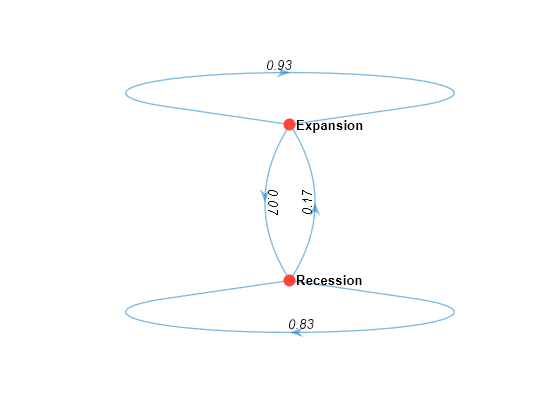
mc is a dtmc object. dtmc normalizes P to create the right-stochastic transition matrix mc.P (each row sums to 1). The element mc.P(1,2) = 0.1659 means that the empirical probability of transitioning to an expansion at time $\mathit{t}$ + 1, given that the US economy is in a recession at time $\mathit{t}$, is 0.1659.

Plot a directed graph of the Markov chain.

graphplot(mc,'LabelEdges',true)

The Markov chain suggests that the current economic state tends to persist, from quarter to quarter.