Filter States of State-Space Model Containing Regression Component
This example shows how to filter states of a time-invariant, state-space model that contains a regression component.
Suppose that the linear relationship between the change in the unemployment rate and the nominal gross national product (nGNP) growth rate is of interest. Suppose further that the first difference of the unemployment rate is an ARMA(1,1) series. Symbolically, and in state-space form, the model is
where:
is the change in the unemployment rate at time t.
is a dummy state for the MA(1) effect.
is the observed change in the unemployment rate being deflated by the growth rate of nGNP ().
is the Gaussian series of state disturbances having mean 0 and standard deviation 1.
is the Gaussian series of observation innovations having mean 0 and standard deviation .
Load the Nelson-Plosser data set, which contains the unemployment rate and nGNP series, among other things.
load Data_NelsonPlosserPreprocess the data by taking the natural logarithm of the nGNP series, and the first difference of each series. Also, remove the starting NaN values from each series.
isNaN = any(ismissing(DataTable),2);       % Flag periods containing NaNs
gnpn = DataTable.GNPN(~isNaN);
u = DataTable.UR(~isNaN);
T = size(gnpn,1);                          % Sample size
Z = [ones(T-1,1) diff(log(gnpn))];
y = diff(u);
Though this example removes missing values, the software can accommodate series containing missing values in the Kalman filter framework.
Specify the coefficient matrices.
A = [NaN NaN; 0 0];
B = [1; 1];
C = [1 0];
D = NaN;
Specify the state-space model using ssm.
Mdl = ssm(A,B,C,D);
Estimate the model parameters. Specify the regression component and its initial value for optimization using the 'Predictors' and 'Beta0' name-value pair arguments, respectively. Restrict the estimate of to all positive, real numbers.
params0 = [0.3 0.2 0.2];
[EstMdl,estParams] = estimate(Mdl,y,params0,'Predictors',Z,...
    'Beta0',[0.1 0.2],'lb',[-Inf,-Inf,0,-Inf,-Inf]);
Method: Maximum likelihood (fmincon)
Sample size: 61
Logarithmic  likelihood:     -99.7245
Akaike   info criterion:      209.449
Bayesian info criterion:      220.003
           |      Coeff       Std Err    t Stat     Prob
----------------------------------------------------------
 c(1)      |  -0.34098       0.29608    -1.15164  0.24948
 c(2)      |   1.05003       0.41377     2.53771  0.01116
 c(3)      |   0.48592       0.36790     1.32079  0.18657
 y <- z(1) |   1.36121       0.22338     6.09358   0
 y <- z(2) | -24.46711       1.60018   -15.29024   0
           |
           |    Final State   Std Dev     t Stat    Prob
 x(1)      |   1.01264       0.44690     2.26592  0.02346
 x(2)      |   0.77718       0.58917     1.31912  0.18713
EstMdl is an ssm model, and you can access its properties using dot notation.
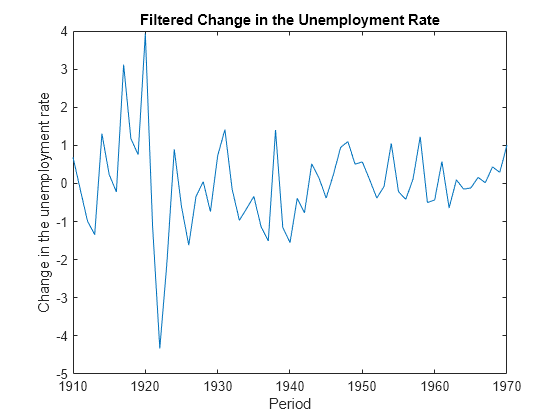
Filter the estimated state-space model. EstMdl does not store the data or the regression coefficients, so you must pass in them in using the name-value pair arguments 'Predictors' and 'Beta', respectively. Plot the estimated, filtered states. Recall that the first state is the change in the unemployment rate, and the second state helps build the first.
filteredX = filter(EstMdl,y,'Predictors',Z,'Beta',estParams(end-1:end));

figure
plot(dates(end-(T-1)+1:end),filteredX(:,1));
xlabel('Period')
ylabel('Change in the unemployment rate')
title('Filtered Change in the Unemployment Rate')
See Also
ssm | estimate | filter | smooth