Generate VEC Model Impulse Responses
This example shows how to generate impulse responses from this vector error-correction model containing the first three lags (VEC(3), see [154], Ch. 6.7):
is a 2-D time series. . is a 2-D series of mean zero Gaussian innovations with covariance matrix
Specify the VEC(3) model autoregressive coefficient matrices , , and , the error-correction coefficient matrix , and the innovations covariance matrix .
B1    = [0.24 -0.08;
         0.00 -0.31];
B2    = [0.00 -0.13;
         0.00 -0.37];
B3    = [0.20 -0.06;
         0.00 -0.34];
C     = [-0.07; 0.17]*[1 -4];
Sigma = [ 2.61 -0.15;
         -0.15  2.31]*1e-5;
Compute the autoregressive coefficient matrices in the VAR(4) model that is equivalent to the VEC(3) model.
B = {B1; B2; B3};
A = vec2var(B,C);
A is a 4-by-1 cell vector containing the 2-by-2 VAR(4) model autoregressive coefficient matrices. Cell A{j} contains the coefficient matrix for lag j in difference-equation notation. The VAR(4) model is in terms of rather than .
Compute the forecast error impulse responses (FEIRs) for the VAR(4) representation. That is, accept the default identity matrix for the innovations covariance. Store the impulse responses for the first 20 periods.
numObs = 20;
IR = cell(2,1); % Preallocation
IR{1} = armairf(A,[],'NumObs',numObs);
IR{1} is a 20-by-2-by-2 array of impulse responses of the VAR representation of the VEC model. Element t,j,k is the impulse response of variable k at time t - 1 in the forecast horizon when variable j received a shock at time 0.
To compute impulse responses, armairf filters a one-standard-deviation innovation shock from one series to itself and all other series. In this case, the magnitude of the shock is 1 for each series.
Compute orthogonalized impulse responses, and supply the innovations covariance matrix. Store the impulse responses for the first 20 periods.
IR{2} = armairf(A,[],'InnovCov',Sigma,'NumObs',numObs);For orthogonalized impulse responses, the innovations covariance governs the magnitude of the filtered shock. IR{2} is commensurate with IR{1}.
Plot the FEIR and the orthogonalized impulse responses for all series.
type = {'FEIR','Orthogonalized'};
for j = 1:2
    figure;
    imp = IR{j};
    subplot(2,2,1);
    plot(imp(:,1,1))
    title(sprintf('%s: y_{1,t}',type{j}));
    ylabel('y_{1,t}');
    xlabel('Period');
    subplot(2,2,2);
    plot(imp(:,1,2))
    title(sprintf('%s: y_{1,t} \\rightarrow y_{2,t}',type{j}));
    ylabel('y_{2,t}');
    xlabel('Period');
    subplot(2,2,3);
    plot(imp(:,2,1))
    title(sprintf('%s: y_{2,t} \\rightarrow y_{1,t}',type{j}));
    ylabel('y_{1,t}');
    xlabel('Period');
    subplot(2,2,4);
    plot(imp(:,2,2))
    title(sprintf('%s: y_{2,t}',type{j}));
    ylabel('y_{2,t}');
    xlabel('Period');
end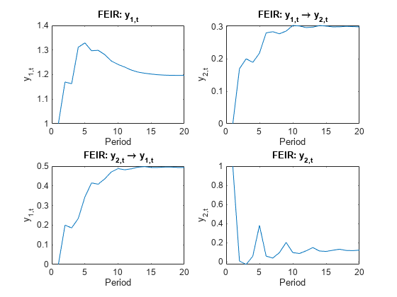
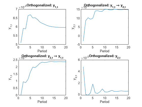
Because the innovations covariance is almost diagonal, the FEIR and orthogonalized impulse responses have similar dynamic behaviors ([154], Ch. 6.7). However, the scale of each plot is markedly different.