Transient Effects in regARIMA Model Simulations
What Are Transient Effects?
When you use automatically generated presample data, you often see transient effects at the beginning of the simulation. This is sometimes called a burn-in period. For stationary error processes, the impulse response function decays to zero over time. This means the starting point of the error simulation is eventually forgotten. To reduce transient effects, you can:
Oversample: generate sample paths that are longer than needed, and discard the beginning samples that show transient effects.
Recycle: use a first simulation to generate presample data for a second simulation.
If the model exhibits nonstationary errors, then the error process does not forget its starting point. By default, all realizations of nonstationary processes begin at zero. For a nonzero starting point, you need to specify your own presample data.
Illustration of Transient Effects on Regression
Transient effects in regression models with ARIMA errors can affect the regression coefficient estimates. The following examples illustrate the behavior of the regression line in models that ignore transient effects and models that account for them.
Transient Effects Are Randomly Spread
This example examines regression lines of regression models with ARMA errors when the transient effects are randomly spread with respect to the joint distribution of the predictor and response.
Specify the regression model with ARMA(2,1) errors:
where is Gaussian with mean 0 and variance 1. Plot the impulse response function.
Mdl0 = regARIMA('AR',{0.9,-0.4},'MA',{0.8},'Beta',2,...
    'Variance',1,'Intercept',3);

figure
impulse(Mdl0)
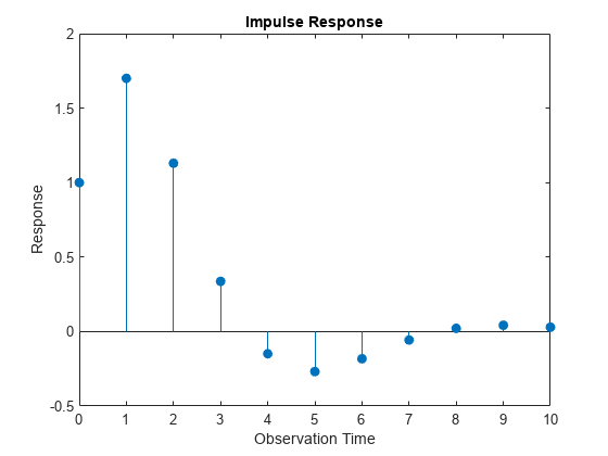
The unconditional disturbances seem to settle after the 10th lag. Therefore, the transient effects end at the 10th lag.
Simulate a univariate, Gaussian predictor series with mean 0 and variance 1. Simulate 100 paths from Mdl0.
rng(5);         % For reproducibility
T = 50;         % Sample size
numPaths = 100; % Number of paths

X = randn(T,1);                                % Full predictor series
Y = simulate(Mdl0,T,'numPaths',numPaths,'X',X); % Full response series

endTrans = 10;
truncX = X((endTrans+1):end);   % Predictor without transient effects
truncY = Y((endTrans+1):end,:); % Response without transient effects
Fit the model to each simulated response path separately for the full and truncated series.
Mdl = regARIMA(2,0,1); % Empty model for estimation
beta1 = zeros(2,numPaths);
beta2 = beta1;

for i = 1:numPaths
    EstMdl1 = estimate(Mdl,Y(:,i),'X',X,'display','off');
    EstMdl2 = estimate(Mdl,truncY(:,i),'X',truncX,'display','off');
    beta1(:,i) = [EstMdl1.Intercept; EstMdl1.Beta];
    beta2(:,i) = [EstMdl2.Intercept; EstMdl2.Beta];
end
beta1 is a 2-by-numPaths matrix containing the estimated intercepts and slopes for each simulated data set. beta2 is a 2-by-numPaths matrix containing the estimated intercepts and slopes for the truncated, simulated data sets.
Compare the simulated regression lines between the full and truncated series. For one of the paths, plot the simulated data and its corresponding regression lines.
betaBar1 = mean(beta1,2);
betaBar2 = mean(beta2,2);
displayresults(betaBar1,betaBar2) % See Supporting Functions section
Transient Effects | Sim. Mean of Intercept | Sim. Mean of Slope =================================================================== Include | 3.08619 | 2.00098 Without | 3.16408 | 1.99455
figure
plot(X,Y(:,1),'.')
hold on
plot(X(1:endTrans),Y(1:endTrans),'ro')
plot([min(X) max(X)],beta1(1,1) + beta1(2,1)*[min(X) max(X)],'b')
plot([min(truncX) max(truncX)],...
    beta2(1,1) + beta2(2,1)*[min(truncX) max(truncX)],'r')
legend('Data','Truncated Data','With Transient Effects',...
    'Without Transient Effects','Location','NorthWest')
xlabel('x')
ylabel('y')
text(0,-3,sprintf('\\beta_0 = %0.4g',beta1(1,1)),'Color',[0,0,1])
text(0,-4,sprintf('\\beta_0 = %0.4g',beta2(1,1)),'Color',[1,0,0])
text(2,-3,sprintf('\\beta_1 = %0.4g',beta1(2,1)),'Color',[0,0,1])
text(2,-4,sprintf('\\beta_1 = %0.4g',beta2(2,1)),'Color',[1,0,0])
hold off
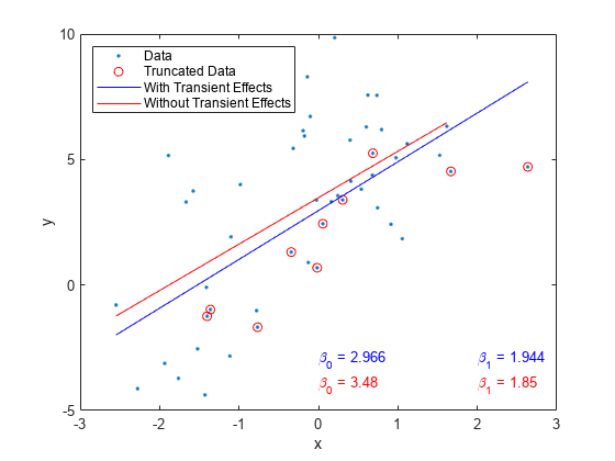
The table in the Command Window displays the simulation averages of the intercept and slope of the regression model. The results suggest the regression line corresponding to the analysis including the full data set is parallel to the regression line corresponding to the truncated data set. In other words, the slope is mostly unaffected by accounting for transient effects, but the intercept is slightly affected.
Supporting Functions
function displayresults(b1,b2)
fprintf('Transient Effects  | Sim. Mean of Intercept    | Sim. Mean of Slope\n')
fprintf('===================================================================\n')
fprintf('Include            | %0.6g                   | %0.6g\n',b1(1),b1(2))
fprintf('Without            | %0.6g                   | %0.6g\n',b2(1),b2(2))
end
Transient Effects Begin the Series
This example examines regression lines of regression models with ARMA errors when the transient effects occur at the beginning of each series.
Specify the regression model with ARMA(2,1) errors:
where is Gaussian with mean 0 and variance 1. Plot the impulse response function.
Mdl0 = regARIMA('AR',{0.9,-0.4},'MA',{0.8},'Beta',2,...
    'Variance',1,'Intercept',3);

figure
impulse(Mdl0)

The unconditional disturbances seem to settle at the 10th lag. Therefore, the transient effects end after the 10th lag.
Simulate a univariate, Gaussian predictor series with mean 0 and variance 1. Simulate 100 paths from Mdl0. Truncate the response and predictor data sets to remove the transient effects.
rng(5);         % For reproducibility
T = 50;         % Sample size
numPaths = 100; % Number of paths

X = linspace(-3,3,T)' + randn(T,1)*0.1;        % Full predictor series
Y = simulate(Mdl0,T,'numPaths',numPaths,'X',X); % Full response series

endTrans = 10;
truncX = X((endTrans+1):end);   % Predictor without transient effects
truncY = Y((endTrans+1):end,:); % Response without transient effects
Fit the model to each simulated response path separately for the full and truncated series.
Mdl = regARIMA(2,0,1); % Empty model for estimation
beta1 = zeros(2,numPaths);
beta2 = beta1;

for i = 1:numPaths
    EstMdl1 = estimate(Mdl,Y(:,i),'X',X,'display','off');
    EstMdl2 = estimate(Mdl,truncY(:,i),'X',truncX,'display','off');
    beta1(:,i) = [EstMdl1.Intercept; EstMdl1.Beta];
    beta2(:,i) = [EstMdl2.Intercept; EstMdl2.Beta];
end
beta1 is a 2-by- numPaths matrix containing the estimated intercepts and slopes for each simulated data set. beta2 is a 2-by- numPaths matrix containing the estimated intercepts and slopes for the truncated, simulated data sets.
Compare the simulated regression lines between the full and truncated series. For one of the paths, plot the simulated data and its corresponding regression lines.
betaBar1 = mean(beta1,2);
betaBar2 = mean(beta2,2);
displayresults(betaBar1,betaBar2) % See Supporting Functions section
Transient Effects | Sim. Mean of Intercept | Sim. Mean of Slope =================================================================== Include | 3.09312 | 2.01796 Without | 3.14734 | 1.98798
figure
plot(X,Y(:,1),'.')
hold on
plot(X(1:endTrans),Y(1:endTrans),'ro')
plot([min(X) max(X)],beta1(1,1) + beta1(2,1)*[min(X) max(X)],'b')
plot([min(truncX) max(truncX)],...
    beta2(1,1) + beta2(2,1)*[min(truncX) max(truncX)],'r')
xlabel('x')
ylabel('y')
legend('Data','Truncated Data','Full Data Regression',...
    'Truncated Data Regression','Location','NorthWest')
text(0,-3,sprintf('\\beta_0 = %0.4g',beta1(1,1)),'Color',[0,0,1])
text(0,-5,sprintf('\\beta_0 = %0.4g',beta2(1,1)),'Color',[1,0,0])
text(2,-3,sprintf('\\beta_1 = %0.4g',beta1(2,1)),'Color',[0,0,1])
text(2,-5,sprintf('\\beta_1 = %0.4g',beta2(2,1)),'Color',[1,0,0])
hold off
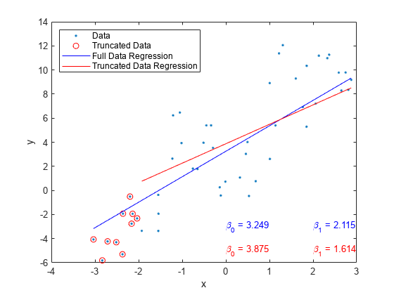
The table in the Command Window displays the simulation averages of the intercept and slope of the regression model. The results suggest that, on average, the regression lines corresponding to the full data and truncated data have slightly different intercepts and slopes. In other words, transient effects slightly affect regression estimates.
The plot displays the data and regression lines for one simulated path. The transient effects seem to affect the results more severely.
Supporting Functions
function displayresults(b1,b2)
fprintf('Transient Effects  | Sim. Mean of Intercept    | Sim. Mean of Slope\n')
fprintf('===================================================================\n')
fprintf('Include            | %0.6g                   | %0.6g\n',b1(1),b1(2))
fprintf('Without            | %0.6g                   | %0.6g\n',b2(1),b2(2))
end