Credit Quality Thresholds
Introduction
An equivalent way to represent transition probabilities is by transforming them into credit quality thresholds. These are critical values of a standard normal distribution that yield the same transition probabilities.
An M-by-N matrix of transition
probabilities TRANS and the corresponding M-by-N matrix
of credit quality thresholds THRESH are related
as follows. The thresholds THRESH(i,j)
are critical values of a standard normal distribution z,
such that
TRANS(i,N) = P[z < THRESH(i,N)],

TRANS(i,j) = P[z < THRESH(i,j)] - P[z < THRESH(i,j+1)], for 1<=j<N
transprobtothresholds and transprobfromthresholds.Compute Credit Quality Thresholds
This example shows how to compute credit quality thresholds.
To compute credit quality thresholds, transition probabilities are required as input. Here is a transition matrix estimated from credit ratings data:
load Data_TransProb
trans = transprob(data)
trans = 8×8
93.1170 5.8428 0.8232 0.1763 0.0376 0.0012 0.0001 0.0017
1.6166 93.1518 4.3632 0.6602 0.1626 0.0055 0.0004 0.0396
0.1237 2.9003 92.2197 4.0756 0.5365 0.0661 0.0028 0.0753
0.0236 0.2312 5.0059 90.1846 3.7979 0.4733 0.0642 0.2193
0.0216 0.1134 0.6357 5.7960 88.9866 3.4497 0.2919 0.7050
0.0010 0.0062 0.1081 0.8697 7.3366 86.7215 2.5169 2.4399
0.0002 0.0011 0.0120 0.2582 1.4294 4.2898 81.2927 12.7167
0 0 0 0 0 0 0 100.0000
Convert the transition matrix to credit quality thresholds using transprobtothresholds.
thresh = transprobtothresholds(trans)
thresh = 8×8

       Inf   -1.4846   -2.3115   -2.8523   -3.3480   -4.0083   -4.1276   -4.1413
       Inf    2.1403   -1.6228   -2.3788   -2.8655   -3.3166   -3.3523   -3.3554
       Inf    3.0264    1.8773   -1.6690   -2.4673   -2.9800   -3.1631   -3.1736
       Inf    3.4963    2.8009    1.6201   -1.6897   -2.4291   -2.7663   -2.8490
       Inf    3.5195    2.9999    2.4225    1.5089   -1.7010   -2.3275   -2.4547
       Inf    4.2696    3.8015    3.0477    2.3320    1.3838   -1.6491   -1.9703
       Inf    4.6241    4.2097    3.6472    2.7803    2.1199    1.5556   -1.1399
       Inf       Inf       Inf       Inf       Inf       Inf       Inf       Inf
Conversely, given a matrix of thresholds, you can compute transition probabilities using transprobfromthresholds. For example, take the thresholds computed previously as input to recover the original transition probabilities.
trans1 = transprobfromthresholds(thresh)
trans1 = 8×8

   93.1170    5.8428    0.8232    0.1763    0.0376    0.0012    0.0001    0.0017
    1.6166   93.1518    4.3632    0.6602    0.1626    0.0055    0.0004    0.0396
    0.1237    2.9003   92.2197    4.0756    0.5365    0.0661    0.0028    0.0753
    0.0236    0.2312    5.0059   90.1846    3.7979    0.4733    0.0642    0.2193
    0.0216    0.1134    0.6357    5.7960   88.9866    3.4497    0.2919    0.7050
    0.0010    0.0062    0.1081    0.8697    7.3366   86.7215    2.5169    2.4399
    0.0002    0.0011    0.0120    0.2582    1.4294    4.2898   81.2927   12.7167
         0         0         0         0         0         0         0  100.0000
Visualize Credit Quality Thresholds
This example shows how to graphically represent the relationship between credit quality thresholds and transition probabilities.
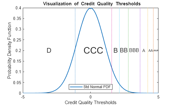
The following code shows the relationship between credit quality thresholds and transition probabilities for the 'CCC' credit rating. In the plot, the thresholds are marked by the vertical lines and the transition probabilities are the area below the standard normal density curve:
load Data_TransProb
trans = transprob(data);
thresh = transprobtothresholds(trans);

xliml = -5;
xlimr = 5;
step = 0.1;
x=xliml:step:xlimr;
thresCCC = thresh(7,:);
labels = {'AAA','AA','A','BBB','BB','B','CCC','D'};

centersX = ([5 thresCCC(2:end)]+[thresCCC(2:end) -5])*0.5;
omag = round(log10(trans(7,:)));
omag(omag>0)=omag(omag>0).^2;
fs = 14+2*omag;

figure
plot(x,normpdf(x),'LineWidth',1.5)
text(centersX(1),0.2,labels{1},'FontSize',fs(1), ...
   'HorizontalAlignment','center')
for i=2:length(labels)
   val = thresCCC(i);
   line([val val],[0 0.4],'LineStyle',':')
   text(centersX(i),0.2,labels{i},'FontSize',fs(i), ...
      'HorizontalAlignment','center')
end
xlabel('Credit Quality Thresholds')
ylabel('Probability Density Function')
title('{\bf Visualization of Credit Quality Thresholds}')
legend('Std Normal PDF','Location','S')
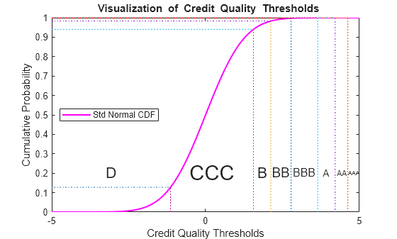
The second plot uses the cumulative distribution function (normcdf) instead. The thresholds are represented by vertical lines. The transition probabilities are given by the distance between horizontal lines.
figure
plot(x,normcdf(x),'m','LineWidth',1.5)
text(centersX(1),0.2,labels{1},'FontSize',fs(1), ...
   'HorizontalAlignment','center')
for i=2:length(labels)
   val = thresCCC(i);
   line([val val],[0 normcdf(val)],'LineStyle',':');
   line([x(1) val],[normcdf(val) normcdf(val)],'LineStyle',':');
   text(centersX(i),0.2,labels{i},'FontSize',fs(i), ...
      'HorizontalAlignment','center')
end
xlabel('Credit Quality Thresholds')
ylabel('Cumulative Probability')
title('{\bf Visualization of Credit Quality Thresholds}')
legend('Std Normal CDF','Location','W')
See Also
transprob | transprobprep | transprobbytotals | bootstrp | transprobgrouptotals | transprobtothresholds | transprobfromthresholds
Topics
- Estimation of Transition Probabilities
- Credit Rating by Bagging Decision Trees
- Forecasting Corporate Default Rates