Optimize Lookup Tables for Periodic Functions

Open Script

This example shows how to use translational and reflectional symmetries in functions in order to optimize lookup tables.

Functions with Symmetry

Functions have symmetry if the functions are unchanged by simple mathematical operations such as translation, rotation, or reflection. When a function has symmetry, the entire range of the function can be generated from a smaller region of the function. After constructing this smaller region, you can translate, reflect, and rotate it to obtain the remainder of the function. This property of functions with symmetry is useful for embedded applications.

Periodic Functions and Discrete Translational Symmetry

Periodic functions are functions with discrete translational symmetry. Discrete translational symmetry means that for the period $T$ , $f(x) = f(x +nT)$ for any integer $n$ . Given any $x$ , you can calculate the value of $f(x)$ by using the identity $f(x) = f(x\ mod\ T)$ . This calculation is equivalent to translating $x$ by an integer multiple of $T$ , such that $0 \le x - nT < T$ .

Periodic Functions and Reflectional Symmetry

Functions can also have reflectional symmetries about lines or points in the Cartesian plane. The most common examples are odd and even functions. Even functions are symmetric about the y-axis, meaning $f(x) = f(-x)$ . Odd functions are symmetric under reflection through the origin, which is expressed as $-f(x) = f(-x)$ . Functions may also be even or odd with respect to other lines and points in the plane. A function that is even with respect to the line $x = C$ will obey $f(C + \Delta x) = f(C - \Delta x)$ . Similarly, a function that is odd with respect to the point $(x,y) = (C, 0)$ will obey $-f(C+\Delta x) = f(C - \Delta x)$ .

Lookup Tables for Symmetric Functions

Lookup tables are used to store the results of expensive calculations. These tables approximate a function by finding the appropriate entry in the table for a given input. Often, the input does not exactly match one that is stored. In this case, further approximation, such as interpolation or rounding, is needed. Further approximation causes numerical errors that can be reduced by creating a larger table. Thus, there is a tradeoff between the accuracy of the approximating lookup table and the memory efficiency of the table.

When approximating a symmetric function, you only need to store a region of the full image of the function. You can construct the remainder by applying the symmetry operations to this region. This process creates smaller, more memory-efficient lookup tables without sacrificing numerical performance.

Use a Lookup Table to Approximate a Superposition of Sinusoids

To demonstrate how to use symmetries to reduce the space in a lookup table, we will use a superposition of two sinusoid functions. This function should be viewed as a non-trivial model that illustrates this concept.

When two or more sinusoids are superimposed, they create a distinct interference pattern that is dependent upon the amplitude and relative phase of each sinusoid. If the ratio of the periods of the sinusoids is rational, then the superposition of the sinusoids is periodic as well, with a period equal to the least common multiple of each period. The interference can lead to a symmetric substructure within each period, though not always.

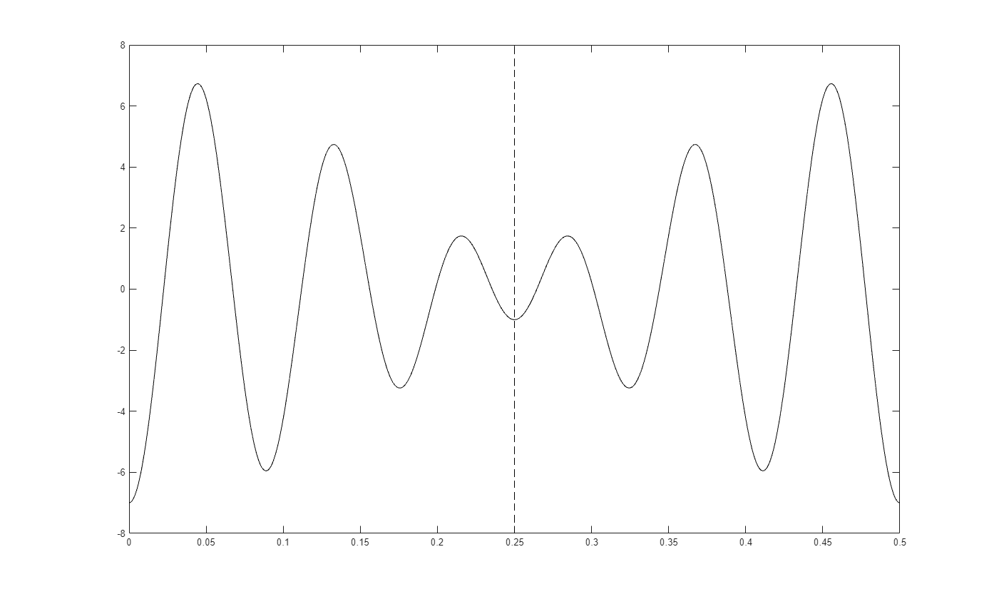
Consider the function $3\times \sin (20\times\pi\times (x - \frac{1}{8})) + 4\times \cos(24\times\pi\times (x-\frac{1}{8}))$ . This function has a period of $\frac{1}{2}$ , as well as an even axis of symmetry about the line $x = \frac{1}{4}$ . You can exploit both of these values to create an efficient lookup table.

The plot below shows the first period of the function, with the axis of even symmetry shown as a dotted vertical line.

h = figure;
x = 0:0.001:0.5;
f = @(x) 3.*sin(20.*pi.*(x - 0.125)) + 4 .* cos(24.*pi.*(x-0.125));
p0 = plot(x, f(x), 'k-');
YLim = [-8, 8];
hold on;
a = h.Children(1);
a.YLim = YLim;
p1 = plot(a, [0.25 0.25], YLim, 'k--');

Consider the case where inputs range from 0 to 10, with a precision of approximately three decimal places. To model this, use an input numeric type with 14 bits, 10 of them fractional.

inputNt = numerictype(0, 14, 10);

Use function approximation to generate a memory-efficient lookup table for any test function. Define the approximation problem by creating a FunctionApproximation.Problem object. Use the solve method to solve the optimization problem.

problem = FunctionApproximation.Problem(f);
problem.InputLowerBounds = 0;
problem.InputUpperBounds = 10;
problem.InputTypes = inputNt;
s1 = problem.solve();
fprintf("Lookup table uses %3.2f Kilobytes\n", s1.totalMemoryUsage ./ 2^10);

|  ID |  Memory (bits) | Feasible | Table Size | Breakpoints WLs | TableData WL | BreakpointSpecification |             Error(Max,Current) | 
|   0 |             92 |        0 |          2 |              14 |           32 |             EvenSpacing |     7.812500e-03, 1.368395e+01 |
|   1 |         163900 |        1 |       5121 |              14 |           32 |             EvenSpacing |     7.812500e-03, 5.173779e-03 |
|   2 |         109276 |        0 |       3414 |              14 |           32 |             EvenSpacing |     7.812500e-03, 1.037254e-02 |
|   3 |          65596 |        0 |       2049 |              14 |           32 |             EvenSpacing |     7.812500e-03, 5.183705e-02 |
|   4 |          81980 |        0 |       2561 |              14 |           32 |             EvenSpacing |     7.812500e-03, 2.058212e-02 |
|   5 |            156 |        0 |          2 |              14 |           64 |             EvenSpacing |     7.812500e-03, 1.368395e+01 |
|   6 |            128 |        0 |          2 |              32 |           32 |             EvenSpacing |     7.812500e-03, 1.368395e+01 |
|   7 |         131164 |        0 |       2049 |              14 |           64 |             EvenSpacing |     7.812500e-03, 5.183710e-02 |
|   8 |             92 |        0 |          2 |              14 |           32 |         EvenPow2Spacing |     7.812500e-03, 1.368395e+01 |
|   9 |          81980 |        0 |       2561 |              14 |           32 |         EvenPow2Spacing |     7.812500e-03, 2.058212e-02 |
|  10 |            156 |        0 |          2 |              14 |           64 |         EvenPow2Spacing |     7.812500e-03, 1.368395e+01 |
|  11 |            128 |        0 |          2 |              32 |           32 |         EvenPow2Spacing |     7.812500e-03, 1.368395e+01 |
|  12 |         138000 |        0 |       3000 |              14 |           32 |          ExplicitValues |     7.812500e-03, 1.037254e-02 |
|  13 |         150006 |        1 |       3261 |              14 |           32 |          ExplicitValues |     7.812500e-03, 7.548735e-03 |
|  14 |         150006 |        0 |       3261 |              14 |           32 |          ExplicitValues |     7.812500e-03, 7.920225e-03 |
|  15 |         150006 |        0 |       3261 |              14 |           32 |          ExplicitValues |     7.812500e-03, 7.920225e-03 |
|  16 |         150006 |        0 |       3261 |              14 |           32 |          ExplicitValues |     7.812500e-03, 7.920225e-03 |
|  17 |         150006 |        0 |       3261 |              14 |           32 |          ExplicitValues |     7.812500e-03, 7.920225e-03 |

Best Solution
|  ID |  Memory (bits) | Feasible | Table Size | Breakpoints WLs | TableData WL | BreakpointSpecification |             Error(Max,Current) |
|  13 |         150006 |        1 |       3261 |              14 |           32 |          ExplicitValues |     7.812500e-03, 7.548735e-03 |

Lookup table uses 146.49 Kilobytes

In this case, the lookup table is large.

Use Function Symmetries to Reduce Size of Lookup Table

Optimizing a lookup table over a smaller range of inputs results in a smaller lookup table, as fewer function values are stored in the table. For this example, only the range for x between 0 and 1/2 needs be stored in the lookup table approximation. Adjusting the input upper and lower bounds and re-solving demonstrates the memory saved.

problem.InputLowerBounds = 0;
problem.InputUpperBounds = 0.25;
s2 = problem.solve();
sprintf("Lookup table uses %1.2f Kilobytes", s2.totalMemoryUsage ./ 2^10)

|  ID |  Memory (bits) | Feasible | Table Size | Breakpoints WLs | TableData WL | BreakpointSpecification |             Error(Max,Current) | 
|   0 |             48 |        0 |          2 |               8 |           16 |             EvenSpacing |     7.812500e-03, 1.262720e+01 |
|   1 |             32 |        0 |          2 |               8 |            8 |             EvenSpacing |     7.812500e-03, 1.262720e+01 |
|   2 |           2080 |        1 |        129 |               8 |           16 |             EvenSpacing |     7.812500e-03, 5.183465e-03 |
|   3 |           1056 |        0 |         65 |               8 |           16 |             EvenSpacing |     7.812500e-03, 2.062116e-02 |
|   4 |             80 |        0 |          2 |               8 |           32 |             EvenSpacing |     7.812500e-03, 1.262720e+01 |
|   5 |             48 |        0 |          2 |               8 |           16 |         EvenPow2Spacing |     7.812500e-03, 1.262720e+01 |
|   6 |             32 |        0 |          2 |               8 |            8 |         EvenPow2Spacing |     7.812500e-03, 1.262720e+01 |
|   7 |           1056 |        0 |         65 |               8 |           16 |         EvenPow2Spacing |     7.812500e-03, 2.062116e-02 |
|   8 |             80 |        0 |          2 |               8 |           32 |         EvenPow2Spacing |     7.812500e-03, 1.262720e+01 |
|   9 |           2544 |        1 |        106 |               8 |           16 |          ExplicitValues |     7.812500e-03, 5.960266e-03 |
|  10 |           2448 |        0 |        102 |               8 |           16 |          ExplicitValues |     7.812500e-03, 1.194193e-02 |
|  11 |           2448 |        0 |        102 |               8 |           16 |          ExplicitValues |     7.812500e-03, 1.106188e-02 |
|  12 |           2712 |        1 |        113 |               8 |           16 |          ExplicitValues |     7.812500e-03, 7.545040e-03 |
|  13 |            144 |        0 |          2 |               8 |           64 |             EvenSpacing |     7.812500e-03, 1.262720e+01 |
|  14 |            128 |        0 |          2 |              32 |           32 |             EvenSpacing |     7.812500e-03, 1.262720e+01 |
|  15 |            144 |        0 |          2 |               8 |           64 |         EvenPow2Spacing |     7.812500e-03, 1.262720e+01 |
|  16 |            128 |        0 |          2 |              32 |           32 |         EvenPow2Spacing |     7.812500e-03, 1.262720e+01 |

Best Solution
|  ID |  Memory (bits) | Feasible | Table Size | Breakpoints WLs | TableData WL | BreakpointSpecification |             Error(Max,Current) |
|   2 |           2080 |        1 |        129 |               8 |           16 |             EvenSpacing |     7.812500e-03, 5.183465e-03 |

ans = 
    "Lookup table uses 2.03 Kilobytes"

Create Lookup Table Block

Use the approximate method to generate a Lookup Table block from the reduced-size lookup table in the previous example.

s2.approximate();

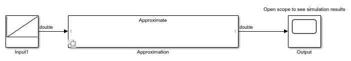
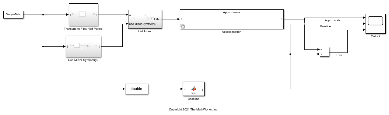
Use the Reduced-Size Lookup Table in a Simulink Model

This model demonstrates how to combine the symmetries of the example function with the lookup table to obtain an accurate approximation. The block diagram illustrates how to use symmetry operations in conjuntion with the lookup table found in the previous example. The lookup table stored in the block named Approximation contains the function values for inputs between 0 and 0.25.

open_system('ModelWithApproximation')

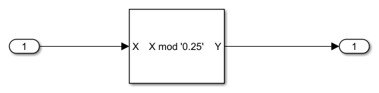
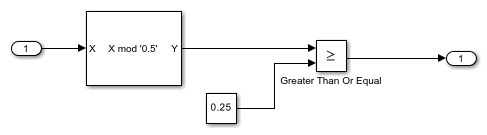
Translate to First Half Period

The subsystem named Translate to First Half Period demonstrates how to use the Modulo by Constant block to reduce the function input to the half open interval [0, 0.25). Note that this block uses the value 0.25 instead of 0.5, because you use both the translational and mirror symmetries of the function for efficiency. Since this block is designed for embedded efficiency, it can reduce this calculation to a cast, as 0.25 is a power of 2.

open_system('ModelWithApproximation/Translate to First Half Period')

Use Mirror Symmetry

To use the mirror symmetry, first check which half of a full period each input lies in. If $x\ mod\ 0.5\ >\ 0.25$ , reflect about the axis of symmetry in the first period. Use the Modulo by Constant block to perform this operation.

open_system('ModelWithApproximation/Use Mirror Symmetry?')

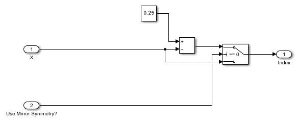
Get the Lookup Table Index

The subsystem named Get Index converts 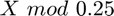$X\ mod\ 0.25$ into a lookup table index. It takes in a Boolean argument to indicate whether you need to reflect about the axis of symmetry. If so, $X mod 0.25$ is subtracted from 0.5 to get the index into the lookup table. Otherwise, is used to get the index.

open_system('ModelWithApproximation/Get Index');

Generate a Floating-Point Baseline

Use a MATLAB function block to generate a suitable floating-point baseline which to compare the lookup table approximation. The body of the function is shown here.

Simulate the System

Create data from 0 to 10 and simulate the model. This range will make it easy to see the repeating interference pattern exhibited by both the lookup table approximation as well as the baseline.

SampleData.signals.values = fi((0:pow2(-10):10)', inputNt);
SampleData.signals.dims = [1,1];
SampleData.time = (0:1:length(SampleData.signals.values)-1)';
sim('ModelWithApproximation');

The scope below compares the approximation and baseline. The error plot shows that the approximation using the compressed lookup table agrees well with the double-precision value of the example function.