Explore Hyperspectral and Multispectral Data in the Hyperspectral Viewer
This example shows how to explore hyperspectral and multispectral data using the Hyperspectral Viewer app. Using the capabilities of the app, you can view the individual bands of a spectral data set as grayscale images. You can also view color composite representations of the data set as RGB, color infrared (CIR), and false-color images. You can also visualize spectral indices of the data. In addition to exploring these visual representations of the spatial dimensions of the data, you can create plots of individual points or small regions of the data along the spectral dimension. These plots, called spectral profiles, can identify elements in the spectral data.
This example requires the Hyperspectral Imaging Library for Image Processing Toolbox™. You can install the Hyperspectral Imaging Library for Image Processing Toolbox from Add-On Explorer. For more information about installing add-ons, see Get and Manage Add-Ons. The Hyperspectral Imaging Library for Image Processing Toolbox requires desktop MATLAB®, as MATLAB® Online™ and MATLAB® Mobile™ do not support the library.
Load Hyperspectral Data into Workspace
For this example, load an aerial hyperspectral data set of an area called Jasper Ridge, captured via the airborne visible/infrared imaging spectrometer (AVIRIS). The data set contains areas of water, land, road, and vegetation. Load the hyperspectral data set into a hypercube object in the MATLAB workspace.
hcube = imhypercube("jasperRidge2_R198.img"); This command creates a hypercube object in the workspace called hcube. The hcube object contains a 100-by-100-by-198 cube of hyperspectral data.
View Hyperspectral Data in Hyperspectral Viewer
Open the Hyperspectral Viewer app. First, click the Apps tab on the MATLAB toolstrip. Then, in the Image Processing and Computer Vision section, click the Hyperspectral Viewer button.
With the app open, you can import hyperspectral data from a file or a hypercube object or data cube from the workspace, using the Import option on the app toolstrip. If you are importing the hyperspectral data from a file, the file must be a NITF file (*.ntf, *.nsf), GeoTIFF metadata file (*.txt) with filename ending in suffix "MTL", ENVI image file (*.img, *.dat, *.raw, *.bil, *.bsq, *.bip) having the same filename as the header file, Hyperion L1R image file (*.L1R), or a multipage TIFF file (*.tif) containing a volume or time series image stack.
Load the hyperspectral data into the app. On the app toolstrip, click Import and select Spectral Object. In the Import from Workspace dialog box, select the hypercube object you loaded into the workspace, hcube. Alternatively, you can also specify a data set when you open the app using the command:
hyperspectralViewer(hcube)
The app displays several views of the Jasper Ridge hyperspectral data. The Bands pane displays the bands of the hyperspectral data as a stack of grayscale images. A second pane includes color composite representations of the hyperspectral data, displaying the False Color tab by default. The Histogram pane displays a histogram of the band currently displayed in the Bands pane. The Spectral Plot pane displays a plot of the spectral dimension of the data by wavelength or by band. (You can rearrange these panes by clicking and dragging them inside the app. To return to the standard pane arrangement, click Default Layout on the app toolstrip.)

View the metadata of the hyperspectral data by selecting the Metadata tab. If the hypercube object is created using the geohypercube function and has geospatial information, you can explore the geospatial information of the hyperspectral data by selecting the Raster Reference tab.

Explore the Spectral Bands
Explore the spectral bands of the Jasper Ridge data set as a stack of grayscale images in the Bands pane. Use the slider at the bottom of the pane to navigate through the images. Because each band isolates a specific range of wavelengths, aspects of the scene might be clearer in some bands than others.

To get a closer look at a band, click Zoom In or Zoom Out in the axes toolbar that appears when you point the cursor over the image.
To improve the contrast of a band image, select the Adjust Contrast option on the app toolstrip. When you do, the app overlays a contrast adjustment window on the histogram of the image, displayed in the Histogram pane. To adjust the contrast, move the window over the histogram or resize the window by clicking and dragging the handles. The app adjusts the contrast using a technique called contrast stretching. In this process, pixel values below a specified value are displayed as black, pixel values above a specified value are displayed as white, and pixel values in between these two values are displayed as shades of gray. The result is a linear mapping of a subset of pixel values to the entire range of grays, from black to white, producing an image of higher contrast. To return to the default view, click Snap Data Range. To remove the contrast adjustment window from the histogram, toggle of the Adjust Contrast option.

Explore Color Representations of Hyperspectral Data
Explore the Jasper Ridge hyperspectral data as a color composite image. To create these color images, Hyperspectral Viewer automatically chooses three of the bands in the hyperspectral dataset to use for the red, green, and blue channels of a color image. The choice of which bands the app uses depends on the type of color representation. The app supports three types of color composite renditions: False Color, RGB, and Color Infrared (CIR). It can be useful to view all of the color composite images because each one uses different bands and can highlight different spectral details, thus increasing the interpretability of the data.
By default, the app displays a false-color representation of the data. False-color composites visualize wavelengths that the human eye cannot see. The tab of the pane identifies the type of the color image, False Color, and the bands that the app used to form it, (19,99,145), in red-green-blue order. The Spectral Plot pane in the app indicates which bands are used. To change these band selections, click and drag the handle of the band indicator in the Spectral Plot. If you choose a different band, the app updates the text in the tab with the new bands and adds the word "Custom", such as, False Color-Custom.

To create the RGB color composite image, the app chooses bands in the visible part of the electromagnetic spectrum. The resulting composite image resembles what the human eye observes naturally. For example, vegetation appears green and water is blue. While RGB composites can appear natural to our eyes, it can be difficult to distinguish subtle differences in features. Natural color images can be low in contrast.

To create the CIR color composite image, the app chooses red, green, and near-infrared wavelengths. Near infrared wavelengths are slightly longer than red, and they are outside of the range visible to the human eye.

Create Spectral Profile Plots of Pixels and Regions
After exploring the grayscale and color visualizations of the hyperspectral data, you can plot points or small regions of the data along the spectral dimension to create spectral profiles. You can plot a single pixel or a region up to 10-by-10 pixels square. Use the Neighborhood Size parameter to specify the region size. When you select a region, the app uses the mean of all the pixels in the region to plot the data. Plotting a region, rather than an individual pixel, can smooth out spectral profiles.
To create spectral plots, click Add Spectral Plot on the app toolstrip, move the cursor over a visualization in the app, and click to select the points or regions. You can make your selections on any of the visualizations provided by the app. Your choice of which visualization to use can depend on which one provides the best view of the particular feature of the data you are interested in. When you make a selection, the app puts a point icon with a black border at that position on all of the visualizations. After selecting all the points, click Add Spectral Plot again to stop adding spectral plots. To delete a point, click on the cross next to the point in the Spectral Plot pane. You can view the statistical information of each spectral plot by selecting the information symbol next to each point in the Spectral Plot pane.
As you select each point, the app plots the data on the Spectral Plot, using a different color to identify each plot. By default, the Spectral Plot also includes a legend identifying the plot for each point. To remove the legend, toggle off the Show Legend option on the app toolstrip. You can clear all the spectral plots including endmembers by selecting Clear All in the app toolstrip.

Plot Endmembers
Since R2024b
Along with the spectral plots of your chosen points, you can plot the endmembers of the hyperspectral data.
On the app toolstrip, specify the number of endmembers to plot using the Number of Endmembers parameter, and select Plot Endmembers.
The app plots the endmembers on the Spectral Plot, using a different color to identify each plot. The app plots the spectral signatures of the endmembers using dotted lines to differentiate them from other spectral plots, and adds point icons with white borders at the positions of the endmember points in the visualizations. You can view the statistical information of each spectral plot by selecting the information symbol next to the corresponding point in the Spectral Plot pane. By default, the Spectral Plot also includes a legend identifying the plot for each endmember point (EM Point). To remove the legend, toggle off the Show Legend option on the app toolstrip. You can clear all the spectral plots, including endmembers, by selecting Clear All in the app toolstrip.

Visualize Spectral Indices of Hyperspectral Data
Since R2023a
You can visualize spectral indices of the hyperspectral data by selecting the desired spectral index from the Spectral Indices section of the app toolstrip. Only the spectral indices that are applicable to the imported hyperspectral data are active.

For example, to visualize the simple ratio (SR) index, select SR from the spectral indices. The app opens a separate pane to visualize the selected spectral indices.

You can create a mask from the spectral index image by using the slider below the image to specify lower and upper thresholds. To go back to the spectral index image without thresholds, select the Reset Threshold option.

You can also select the Custom index, and define a custom spectral index for the imported hyperspectral data. You must define a custom index compatible with the customSpectralIndex function. Specify the custom index formula as a function handle and the wavelengths for the custom index computation as a numeric vector. The wavelengths must be unique, must be specified in nanometers, and must lie within the range of wavelengths within the hyperspectral data cube.


Export to Workspace
Since R2023b
From the app toolstrip, select Export to Workspace. You can choose to export one of these options.
False Color, RGB, CIR Color Bands
Spectral Indices
Spectral Signatures

If you select the False Color, RGB, CIR Color Bands option, in the Export to Workspace dialog box, select and name the color representations that you want to export to the workspace. The app exports the selected color representations to the MATLAB workspace as numeric arrays.

If you select the Spectral Indices option, in the Export to Workspace dialog box, select and name the spectral indices and thresholded spectral index masks that you want to export to the workspace. The app exports the selected spectral indices and thresholded spectral index masks to the MATLAB workspace as numeric arrays.

If you select the Spectral Signatures option, in the Export to Workspace dialog box, select and name the spectral signatures, plotted in the spectral plots or plotted as endmembers, that you want to export to the workspace. The app exports the selected spectral signatures to the MATLAB workspace as numeric vectors.

Explore Multispectral Data in Hyperspectral Viewer
Since R2025a
Download Landsat 8 multispectral data.
zipfile = "LC08_L1TP_113082_20211206_20211215_02_T1.zip";
landsat8Data_url = "https://ssd.mathworks.com/supportfiles/image/data/" + zipfile;
hyper.internal.downloadLandsatDataset(landsat8Data_url,zipfile)
filepath = fullfile("LC08_L1TP_113082_20211206_20211215_02_T1","LC08_L1TP_113082_20211206_20211215_02_T1_MTL.txt");
Read a multispectral image into the workspace with geospatial information as a multicube object, mcube.
mcube = geomulticube(filepath);
In the Hyperspectral Viewer app, you can import multispectral data from a file or from a multicube object or data cube in the workspace, by using the Import option on the app toolstrip. If you are importing the multispectral data from a file, the file must be a GeoTIFF metadata file (.txt) with a filename ending in the suffix "MTL", ASTER image file (.hdf), a Sentinel-2 file (.safe), or a multipage TIFF file (.tif) containing a volume or time series image stack.
Load the multispectral data into the app. On the app toolstrip, click Import and select Spectral Object. In the Import from Workspace dialog box, select the multicube object you loaded into the workspace mcube. Alternatively, you can specify a data set and a target resolution when you open the app using this command:
hyperspectralViewer(mcube,resolution)
The app gathers the data cube of the multispectral data for visualization. Thus, you must resample the multispectral data to a uniform resolution. In the Import from Workspace dialog box, select one of the data resolutions available in the multicube object as the uniform target resolution.

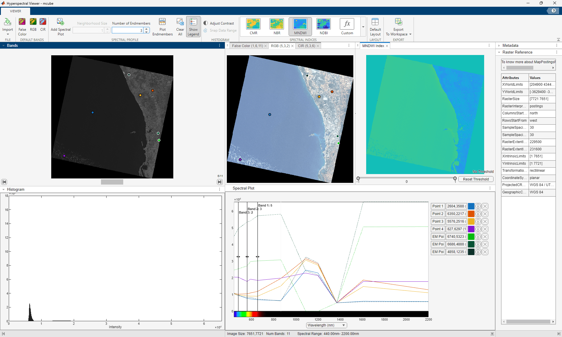
In the Bands pane, explore images in individual spectral bands of the multispectral image. In the Histogram pane, explore the histogram of the band currently displayed in the Bands pane. Visualize the false-color, RGB, and CIR color representations of the multispectral data. You can select points in the color representations to plot the spectral signatures and also plot endmembers in the Spectral Plot pane. You can also visualize spectral indices of the multispectral data. View the metadata of the multispectral data by selecting the Metadata tab. If the multicube object was created using the geomulticube function and has geospatial information, you can explore the geospatial information of the multispectral data by selecting the Raster Reference tab. Export the color representations, spectral signatures, endmember signatures, and spectral indices by selecting Export to Workspace in the app toolstrip.
See Also
Hyperspectral
Viewer | hypercube | multicube