quantum.gate.QuantumMeasurement Class

Namespace: quantum.gate

Measurement result of quantum circuit

Since R2023a

Installation Required: This functionality requires MATLAB Support Package for Quantum Computing.

Description

A QuantumMeasurement object represents the measurement result of a quantum circuit, either by running the circuit remotely on a quantum device or by simulating the circuit locally with random sampling. This object contains information about the counts of all measured states of the n qubits of the circuit.

Creation

• Use run to run a circuit remotely on a quantum device and fetch the finished task using fetchOutput to return a QuantumMeasurement object.

• Use randsample on a QuantumState object that represents the quantum state of the qubits of a circuit. randsample randomly samples this state locally (with a specified number of shots) and returns the measurement result as a QuantumMeasurement object.

Properties

MeasuredStates — Measured states in Z basis

string array

Measured states in the Z basis, returned as a string array.

Attributes:

GetAccess	public
SetAccess	private

Counts — Counts of measured states

vector of positive integers or NaN values

Counts of measured states, returned as a vector of positive integers or NaN values.

• When you use randsample on a QuantumState object, the Counts property of the returned QuantumMeasurement object is a vector of positive integers. Each element of this vector represents the number of counts of each measured state.

• When you use the run function and the remote device provider does not return the number of counts of each measured state, the Counts property of the returned QuantumMeasurement object is a vector of NaN values. Otherwise, the Counts property is a vector of positive integers.

Attributes:

GetAccess	public
SetAccess	private

Probabilities — Estimated probabilities of measured states

vector of real numbers

Estimated probabilities of measured states, returned as a vector of real numbers. Each element of this vector represents how often each state was measured.

Attributes:

GetAccess	public
SetAccess	private

NumQubits — Number of qubits

positive integer scalar

Number of qubits, returned as a positive integer scalar.

Attributes:

GetAccess	public
SetAccess	private

Methods

Public Methods

histogram	Histogram plot of possible states
probability	Probability of measuring qubits in given state
querystates	Query possible states

Examples

Simulate Circuit Locally with Random Sampling

Create a quantum circuit that consists of three x-axis rotation gates. The first gate acts on qubit 1 with rotation angle pi/4, the second gate acts on qubit 2 with rotation angle pi/2, and the third gate acts on qubit 3 with rotation angle 3*pi/4.

g = rxGate(1:3,pi/4*(1:3));
c = quantumCircuit(g);

Simulate this circuit using the default initial state, where all qubits are in the $$|0\rangle$$ state. After running the circuit, randomly sample the quantum state with 100 shots and return the resulting simulated measurement.

s = simulate(c);
m = randsample(s,100)

m = 

  QuantumMeasurement with properties:

    MeasuredStates: [7×1 string]
            Counts: [7×1 double]
     Probabilities: [7×1 double]
         NumQubits: 3

Show the counts and estimated probabilities of the measured states.

table(m.Counts,m.Probabilities,m.MeasuredStates, ...
    VariableNames=["Counts","Probabilities","States"])

ans =

  7×3 table

    Counts    Probabilities    States
    ______    _____________    ______

       6          0.06         "000" 
      33          0.33         "001" 
       5          0.05         "010" 
      40           0.4         "011" 
       5          0.05         "101" 
       3          0.03         "110" 
       8          0.08         "111" 

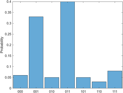
Plot the histogram of the measurement result to show each measured state and its estimated probability.

histogram(m)

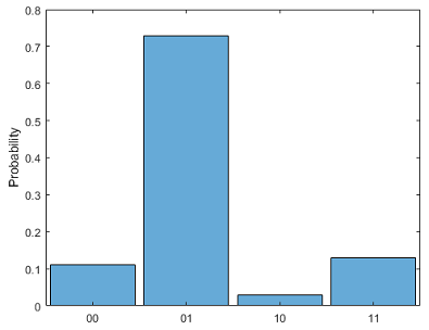
You can also specify which qubits to plot in the histogram. The histogram shows the measured states of the specified qubits (where the other qubits can be in any state) and their corresponding probability distributions (where the probabilities of the other qubits being in any state are combined).

For example, specify qubits 1 and 3 to plot in the histogram. This histogram shows the measured states $$|00\rangle$$, $$|01\rangle$$, $$|10\rangle$$, and $$|11\rangle$$, where their corresponding probabilities are 0.11, 0.73, 0.03, and 0.13.

histogram(m,[1 3])

Query each measured state and its estimated probability.

[states,probabilities] = querystates(m)

states = 

  7×1 string array

    "000"
    "001"
    "010"
    "011"
    "101"
    "110"
    "111"


probabilities =

    0.0600
    0.3300
    0.0500
    0.4000
    0.0500
    0.0300
    0.0800

You can also specify which qubits to query when using querystates.

[states,probabilities] = querystates(m,[1 3])

states = 

  4×1 string array

    "00"
    "01"
    "10"
    "11"


probabilities =

    0.1100
    0.7300
    0.0300
    0.1300

Run Circuit Remotely on AWS Quantum Device

Create a quantum circuit that consists of a Hadamard gate and a controlled X gate to entangle two qubits.

gates = [hGate(1); cxGate(1,2)];
c = quantumCircuit(gates);

Connect to a remote quantum device through AWS^®. Create a task that runs the circuit on the device.

dev = quantum.backend.QuantumDeviceAWS("Lucy");
task = run(c,dev);

Wait for the task to finish. Retrieve the result of running the circuit on the device.

wait(task)
m = fetchOutput(task)

m = 

  QuantumMeasurement with properties:

    MeasuredStates: [4×1 string]
            Counts: [4×1 double]
     Probabilities: [4×1 double]
         NumQubits: 2

Show the measurement result of running the circuit. Due to the noise in the physical quantum device, the $$|01\rangle$$ and $$|10\rangle$$ states can appear as measurements.

table(m.Counts,m.Probabilities,m.MeasuredStates, ...
    VariableNames=["Counts","Probabilities","States"])

ans =

  4×3 table

    Counts    Probabilities    States
    ______    _____________    ______

      46          0.46          "00" 
       9          0.09          "10" 
       3          0.03          "01" 
      42          0.42          "11" 

Run Circuit Remotely on IBM Quantum Device Without and With Error Mitigation

Create a quantum circuit that consists of a Hadamard gate and a controlled X gate to entangle two qubits.

gates = [hGate(1); cxGate(1,2)];
c = quantumCircuit(gates);

Connect to a remote quantum device through the IBM^® Qiskit^® Runtime Services. Create a task that runs the circuit on the device without error mitigation.

dev = quantum.backend.QuantumDeviceIBM("ibmq_qasm_simulator");
task = run(c,dev,NumShots=500,UseErrorMitigation=false);

Wait for the task to finish. Retrieve the result of running the circuit on the device.

wait(task)
m = fetchOutput(task)

m = 

  QuantumMeasurement with properties:

    MeasuredStates: [4×1 string]
            Counts: [4×1 double]
     Probabilities: [4×1 double]
         NumQubits: 2

Show the measurement result of running the circuit. Due to the noise in the physical quantum device, the $$|01\rangle$$ and $$|10\rangle$$ states can appear as measurements.

table(m.Probabilities,m.MeasuredStates, ...
    VariableNames=["Probabilities","States"])

ans =

  4×2 table

    Probabilities    States
    _____________    ______
        0.536         "00" 
        0.018         "10" 
        0.024         "01" 
        0.422         "11"
       

Next, create a task that runs the circuit on the same device by applying quantum error mitigation. The error mitigation is a collection of tools and methods to process measurement results that are aimed at reducing the effects of measurement errors.

task = run(c,dev,NumShots=500,UseErrorMitigation=true);

Wait for the task to finish. Retrieve the result of running the circuit on the device.

wait(task)
m = fetchOutput(task)

m = 

  QuantumMeasurement with properties:

    MeasuredStates: [4×1 string]
            Counts: [4×1 double]
     Probabilities: [4×1 double]
         NumQubits: 2

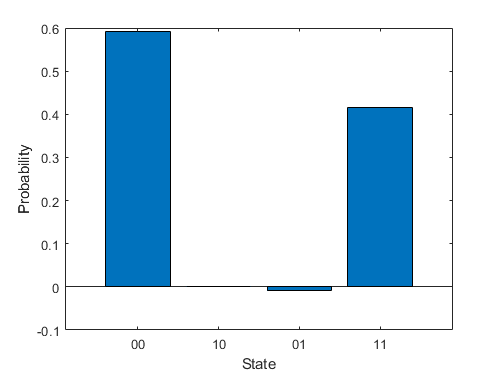
Show the measurement result of running the circuit with error mitigation. Here, the estimated probabilities of the $$|01\rangle$$ and $$|10\rangle$$ states are closer to 0.

table(m.Probabilities,m.MeasuredStates, ...
    VariableNames=["Probabilities","States"])

ans =

  4×2 table

    Probabilities    States
    _____________    ______
        0.59254       "00" 
       0.001586       "10" 
     -0.0094173       "01" 
         0.4153       "11" 

Plot this measurement result in a bar graph.

bar(m.States,m.Probabilities)
xlabel("State")
ylabel("Probability")

Version History

Introduced in R2023a