Dynamics of Damped Cantilever Beam
This example shows how to include damping in the transient analysis of a simple cantilever beam.
The damping model is basic viscous damping distributed uniformly through the volume of the beam. The beam is deformed by applying an external load at the tip of the beam and then released at time . This example does not use any additional loading, so the displacement of the beam decreases as a function of time due to the damping. The example uses plane-stress modal, static, and transient analysis in its three-step workflow:
Perform modal analysis to compute the fundamental frequency of the beam and to speed up computations for transient analysis.
Find the static solution of the beam with a vertical load at the tip to use as an initial condition for transient analysis.
Perform transient analysis with and without damping.
Damping is typically expressed as a percentage of critical damping, , for a selected vibration frequency. This example uses , which is three percent of critical damping.
The example specifies values of parameters using the imperial system of units. You can replace them with values specified in the metric system. If you do so, ensure that you specify all values throughout the example using the same system.
Modal Analysis
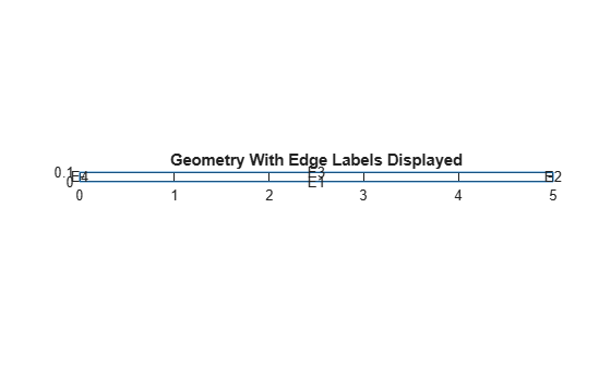
Create the geometry of a beam which is 5 inches long and 0.1 inches thick.
width = 5;
height = 0.1;
gdm = [3;4;0;width;width;0;0;0;height;height];
g = decsg(gdm,'S1',('S1')');
Plot the geometry with the edge labels.
figure;
pdegplot(g,EdgeLabels="on");
axis equal
title("Geometry With Edge Labels Displayed")
Create an femodel object for structural modal analysis and include the geometry in the model.
model = femodel(AnalysisType="structuralModal", ....
                Geometry=g);
Define a maximum element size so that there are five elements through the beam thickness. Generate a mesh.
hmax = height/5;
model = generateMesh(model,Hmax=hmax);
Specify Young's modulus, Poisson's ratio, and the mass density of steel.
E = 3.0e7;
nu = 0.3;
rho = 0.3/386;
model.MaterialProperties = ...
    materialProperties(YoungsModulus=E, ...
                       PoissonsRatio=nu, ...
                       MassDensity=rho);
Specify that the left edge of the beam is a fixed boundary.
model.EdgeBC(4) = edgeBC(Constraint="fixed");Solve the problem for the frequency range from 0 to 1e5. The recommended approach is to use a value that is slightly smaller than the expected lowest frequency. Thus, use -0.1 instead of 0.
res = solve(model,FrequencyRange=[-0.1,1e5]')
res =
  ModalStructuralResults with properties:

    NaturalFrequencies: [8×1 double]
            ModeShapes: [1×1 FEStruct]
                  Mesh: [1×1 FEMesh]
By default, the solver returns circular frequencies.
modeID = 1:numel(res.NaturalFrequencies);
Express the resulting frequencies in Hz by dividing them by 2π. Display the frequencies in a table.
tmodalResults = table(modeID.',res.NaturalFrequencies/(2*pi));
tmodalResults.Properties.VariableNames = {'Mode','Frequency'};
disp(tmodalResults)
Mode Frequency
____ _________
1 126.94
2 794.05
3 2216.8
4 4325.3
5 7110.7
6 9825.9
7 10551
8 14623
Compute the analytical fundamental frequency (Hz) using the beam theory.
I = height^3/12;
freqAnalytical = 3.516*sqrt(E*I/(width^4*rho*height))/(2*pi)
freqAnalytical =
126.9498
Compare the analytical result with the numerical result.
freqNumerical = res.NaturalFrequencies(1)/(2*pi)
freqNumerical =
126.9416
Compute the period corresponding to the lowest vibration mode.
longestPeriod = 1/freqNumerical
longestPeriod =
0.0079
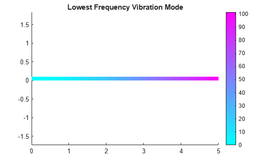
Plot the y-component of the solution for the lowest beam frequency.
figure;
pdeplot(res.Mesh,XYData=res.ModeShapes.uy(:,1))
title("Lowest Frequency Vibration Mode")
axis equal
Initial Displacement from Static Solution
The beam is deformed by applying an external load at its tip and then released at time . Find the initial condition for the transient analysis by using the static solution of the beam with a vertical load at the tip.
Switch the analysis type of the model to static structural analysis.
model.AnalysisType="structuralStatic";Specify the plane-stress problem type.
model.PlanarType = "planeStress";Apply the static vertical load on the right side of the beam.
model.EdgeLoad(2) = edgeLoad(SurfaceTraction=[0;1]);
Solve the problem. The resulting static solution serves as an initial condition for transient analysis.
Rstatic = solve(model)
Rstatic =
  StaticStructuralResults with properties:

      Displacement: [1×1 FEStruct]
            Strain: [1×1 FEStruct]
            Stress: [1×1 FEStruct]
    VonMisesStress: [6511×1 double]
              Mesh: [1×1 FEMesh]
Transient Analysis
Perform the transient analysis of the cantilever beam with and without damping. Use the modal superposition method to speed up computations.
Switch the analysis type of the model to transient structural analysis.
model.AnalysisType = "structuralTransient";Remove all previously assigned loads on the beam.
model.EdgeLoad = [];
Specify the initial condition by using the static solution.
model.FaceIC = faceIC(Displacement=Rstatic);
Solve the undamped transient model for three full periods corresponding to the lowest vibration mode.
tlist = 0:longestPeriod/100:3*longestPeriod;
resT = solve(model,tlist,ModalResults=res);
Interpolate the displacement at the tip of the beam.
intrpUt = interpolateDisplacement(resT,[5;0.05]);
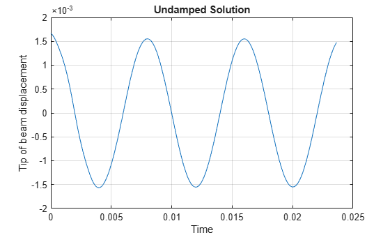
The displacement at the tip is a sinusoidal function of time with amplitude equal to the initial y-displacement. This result agrees with the solution to the simple spring-mass system.
plot(resT.SolutionTimes,intrpUt.uy)
grid on
title("Undamped Solution")
xlabel("Time")
ylabel("Tip of beam displacement")
Now solve the model with damping equal to 3% of critical damping.
zeta = 0.03;
omega = 2*pi*freqNumerical;
resT = solve(model,tlist, ...
             ModalResults=res, ...
             DampingZeta=zeta);
Interpolate the displacement at the tip of the beam.
intrpUt = interpolateDisplacement(resT,[5;0.05]);
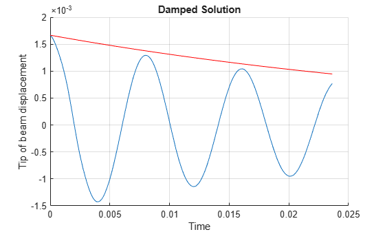
The y-displacement at the tip is a sinusoidal function of time with amplitude exponentially decreasing with time.
figure
hold on
plot(resT.SolutionTimes,intrpUt.uy)
plot(tlist,intrpUt.uy(1)*exp(-zeta*omega*tlist),Color="r")
grid on
title("Damped Solution")
xlabel("Time")
ylabel("Tip of beam displacement")