Thermal Stress Analysis of Jet Engine Turbine Blade
This example shows how to compute the thermal stress and deformation of a turbine blade in its steady-state operating condition. The blade has interior cooling ducts. The cool air flowing through the ducts maintains the temperature of the blade within the limit for its material. This feature is common in modern blades.
A turbine is a component of the jet engine. It is responsible for extracting energy from the high-temperature and high-pressure gas produced in the combustion chamber and transforming it into rotational motion to produce thrust. The turbine is a radial array of blades typically made of nickel alloys. These alloys resist the extremely high temperatures of the gases. At such temperatures, the material expands significantly, producing mechanical stress in the joints and significant deformations of several millimeters. To avoid mechanical failure and friction between the tip of the blade and the turbine casing, the blade design must account for the stress and deformations.
The example shows a three-step workflow:
Perform structural analysis accounting only for pressure of the surrounding gases while ignoring thermal effects.
Compute the thermal stress while ignoring the pressure.
Combine the pressure and thermal stress.
Pressure Loading
The blade experiences high pressure from the surrounding gases. Compute the stress caused only by this pressure.
First, create an femodel object for static structural analysis and include the geometry of a turbine blade.
model = femodel(AnalysisType="structuralStatic", ...
                Geometry="Blade.stl");
Plot the geometry with face labels.
pdegplot(model,FaceLabels="on",FaceAlpha=0.5)
Generate a mesh with the maximum element size 0.01.
model = generateMesh(model,Hmax=0.01);
Specify Young's modulus, Poisson's ratio, and the coefficient of thermal expansion for nickel-based alloy (NIMONIC 90).
E = 227E9; % in Pa
CTE = 12.7E-6; % in 1/K
nu = 0.27;

model.MaterialProperties = ...
    materialProperties(YoungsModulus=E, ...
                       PoissonsRatio=nu, ...
                       CTE=CTE);
Specify that the face of the root that is in contact with other metal is fixed.
model.FaceBC(3) = faceBC(Constraint="fixed");Specify the pressure load on the pressure and suction sides of the blade. This pressure is due to the high-pressure gas surrounding these sides of the blade.
p1 = 5e5; %in Pa
p2 = 4.5e5; %in Pa

model.FaceLoad(11) = faceLoad(Pressure=p1); % Pressure side
model.FaceLoad(10) = faceLoad(Pressure=p2);  % Suction side
Solve the structural problem.
Rs = solve(model);
Plot the von Mises stress and the displacement. Specify a deformation scale factor of 100 to better visualize the deformation.
figure
pdeplot3D(Rs.Mesh, ...
          ColorMapData=Rs.VonMisesStress, ...
          Deformation=Rs.Displacement, ...
          DeformationScaleFactor=100)
view([116,25]);

The maximum stress is around 100 Mpa, which is significantly below the elastic limit.
Thermal Stress
Determine the temperature distribution and compute the stress and deformation due to thermal expansion only. This part of the example ignores the pressure.
First, switch the analysis type of the model to the steady-state thermal analysis.
model.AnalysisType = "thermalSteady";Assuming that the blade is made of nickel-based alloy (NIMONIC 90), specify the thermal conductivity.
kapp = 11.5; % in W/m/K
model.MaterialProperties = ...
    materialProperties(ThermalConductivity=kapp);
Convective heat transfer between the surrounding fluid and the faces of the blade defines the boundary conditions for this problem. The convection coefficient is greater where the gas velocity is higher. Also, the gas temperature is different around different faces. The temperature of the interior cooling air is , while the temperature on the pressure and suction sides is .
% Interior cooling
model.FaceLoad([15 12 14]) = ...
    faceLoad(ConvectionCoefficient=30, ...
             AmbientTemperature=150);
% Pressure side
model.FaceLoad(11) = ...
    faceLoad(ConvectionCoefficient=50, ...
             AmbientTemperature=1000);
% Suction side
model.FaceLoad(10) = ...
    faceLoad(ConvectionCoefficient=40, ...
             AmbientTemperature=1000);
% Tip
model.FaceLoad(13) = ...
    faceLoad(ConvectionCoefficient=20, ...
             AmbientTemperature=1000);
% Base (exposed to hot gases)
model.FaceLoad(1) = ...
    faceLoad(ConvectionCoefficient=40, ...
             AmbientTemperature=800);
% Root in contact with hot gases
model.FaceLoad([6 9 8 2 7]) = ...
    faceLoad(ConvectionCoefficient=15, ...
             AmbientTemperature=400);
The boundary condition for the faces of the root in contact with other metal is a thermal contact that can be modeled as convection with a very large coefficient (around for metal-metal contact).
% Root in contact with metal
model.FaceLoad([3 4 5]) = ...
    faceLoad(ConvectionCoefficient=1000, ...
             AmbientTemperature=300);
Solve the thermal problem.
Rt = solve(model);
Plot the temperature distribution. The temperature between the tip and the root ranges from around to . The exterior gas temperature is . The interior cooling is efficient: it significantly lowers the temperature.
figure
pdeplot3D(Rt.Mesh,ColorMapData=Rt.Temperature)
view([130,-20]);

Now, compute the stress and deformation due to thermal expansion. First, switch the analysis type of the model to the static structural analysis.
model.AnalysisType = "structuralStatic";Specify Young's modulus, Poisson's ratio, and the coefficient of thermal expansion for nickel-based alloy (NIMONIC 90).
model.MaterialProperties = ...
    materialProperties(YoungsModulus=E, ...
                       PoissonsRatio=nu, ...
                       CTE=CTE);
Specify the reference temperature.
model.ReferenceTemperature = 300; %in degrees C
model.CellLoad = cellLoad(Temperature=Rt);
Specify the boundary condition.
model.FaceBC(3) = faceBC(Constraint="fixed");Solve the thermal stress problem.
Rts = solve(model);
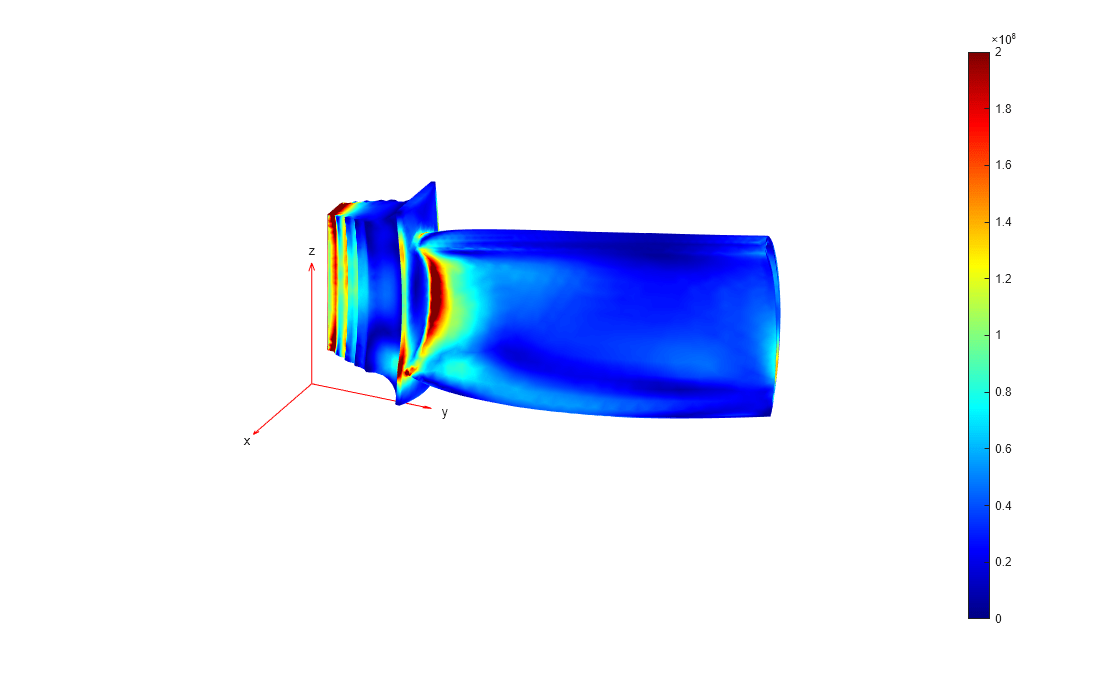
Plot the von Mises stress and the displacement. Specify a deformation scale factor of 100 to better visualize the deformation. The stress concentrates in the constrained root because it cannot freely expand, and also in the junction between the blade and the root.
figure("units","normalized","outerposition",[0 0 1 1]);
pdeplot3D(Rts.Mesh, ...
          ColorMapData=Rts.VonMisesStress, ...
          Deformation=Rts.Displacement, ...
          DeformationScaleFactor=100)
clim([0, 200e6])
view([116,25]);
Evaluate the displacement at the tip. In the design of the cover, this displacement must be taken into account to avoid friction between the cover and the blade.
max(Rts.Displacement.Magnitude)
ans =
0.0015
Combined Pressure Loading and Thermal Stress
Compute the stress and deformations caused by the combination of thermal and pressure effects.
Add the pressure load on the pressure and suction sides of the blade. This pressure is due to the high-pressure gas surrounding these sides of the blade.
% Pressure side
model.FaceLoad(11) = faceLoad(Pressure=p1);
% Suction side
model.FaceLoad(10) = faceLoad(Pressure=p2);
Solve the problem.
Rc = solve(model);
Plot the von Mises stress and the displacement. Specify a deformation scale factor of 100 to better visualize the deformation.
figure("units","normalized","outerposition",[0 0 1 1]);
pdeplot3D(Rc.Mesh,...
          ColorMapData=Rc.VonMisesStress, ...
          Deformation=Rc.Displacement, ...
          DeformationScaleFactor=100)
clim([0, 200e6])
view([116,25]);

Evaluate the maximum stress and maximum displacement. The displacement is almost the same as for the thermal stress analysis, while the maximum stress, 854 MPa, is significantly higher.
max(Rc.VonMisesStress)
ans =
9.5085e+08
max(Rc.Displacement.Magnitude)
ans =
0.0015