Model a Series RLC Circuit

Open Model

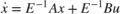
Physical systems can be described as a series of differential equations in an implicit form, $F\left(t,x,\dot{\left\lbrace x\right\rbrace } \right)=0$ , or in the implicit state-space form $E\dot{x} =A\;x+B\;u\;$

If $E$ is nonsingular, then the system can be easily converted to a system of ordinary differential equations (ODEs) and solved as such:

$\dot{x} =\left(E^{-1} A\right)x+\left(E^{-1} B\right)u$

Many times, states of a system appear without a direct relation to their derivatives, usually representing physical conservation laws. For example:

$\begin{array}{l}\dot{x_1 } =x_2 \\0\;=x_1 +x_2 \end{array}$

In this case, $E$ is singular and cannot be inverted. This class of systems are commonly called descriptor systems and the equations are called differential-algebraic equations (DAEs).

Series RLC Circuit

Consider the simple series RLC circuit.

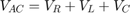
From Kirchoff's Voltage Law, the voltage drop across the circuit is equalt to the sum of the voltage drop across each of its elements:

$V_{AC} = V_R+V_L+V_C$

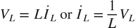
From Kirchoff's Current Law:

$I_{AC}=I_R=I_L=I_C$

where the subscripts $R$ , $L$ , and $C$ denote the resistance, inductance, and capacitance respectively.

$V_{R} =I\left(t\right)R$

$V_L =L\dot{I_L }$ or $\dot{I_L } = \frac{1}{L}V_L$

$V_C =V_{AC} \left(0\right)+\int_0^t I_C \left(\tau \right)d\tau$ or $\dot{V_c } =\frac{1}{C}I_c$

In Implicit State-Space Form

Model the system in Simulink with $R=10\;\Omega$ , $L=1\times {10}^{-6} \;H$ , $C=1\times {10}^{-4} F$ to find the voltage across the resistor $V_R$ . To use the Descriptor State-Space block, the system can be written in the implicit, or descriptor, state-space form $E\dot{x}=Ax+Bu$ as shown below.

$\left\lbrack \begin{array}{ccccc}1 & 0 & 0 & 0 & 0\\0 & 0 & 0 & 0 & 0\\0
& 0 & 0 & 0 & 0\\0 & 0 & 0 & 1 & 0\\0 & 0 & 0 & 0 & 0\end{array}\right\rbrack
\left\lbrack \begin{array}{c}\dot{V_C } \\\dot{V_L } \\\dot{V_R } \\\dot{I_L
} \\\dot{I_{AC} } \end{array}\right\rbrack =\left\lbrack \begin{array}{ccccc}0
& 0 & 0 & \frac{1}{C} & 0\\1 & 1 & 1 & 0 & 0\\0 & 0 & -1 & R & 0\\0 & \frac{1}{L}
& 0 & 0 & 0\\0 & 0 & 0 & 1 & -1\end{array}\right\rbrack \left\lbrack \begin{array}{c}V_C
\\V_L \\V_R \\I_L \\I_{AC} \end{array}\right\rbrack +\left\lbrack \begin{array}{c}0\\-1\\0\\0\\0\end{array}\right\rbrack
V_{AC}$

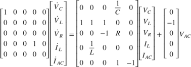
where $x = {\left\lbrack \begin{array}{ccccc}V_C &V_L& V_R& I_L& I_{AC}\end{array}\right\rbrack}^T$ is the state vector.

Set $C=\left\lbrack \begin{array}{ccccc}0&0& 1& 0&0\end{array}\right\rbrack$ since the voltage across the resistor is being measured.

Compare this to modeling the system with an algebraic loop in order to find $V_R$ .

The simulation of both models produces identical results. However, the Descriptor State-Space block allows you to make a simpler block diagram and avoid algebraic loops.

Model a Series RLC Circuit

Series RLC Circuit

In Implicit State-Space Form

See Also