Choose a Fixed-Step Solver

This example shows an algorithmic method of selecting an appropriate fixed-step solver for your model. For simulation workflows in Simulink^®, the default setting for the Solver parameter in the Model Configuration Parameters is auto. The heuristics used by Simulink to select a variable-step solver is shown in the figure below.

When to Use a Fixed-Step Solver

One common case to use a fixed-step solver is for workflows where you plan to generate code from your model and run the code on a real-time system.

With a variable-step solver, the step size can vary from step to step, depending on the model dynamics. In particular, a variable-step solver increases or reduces the step size to meet the error tolerances that you specify and as such, the variable step sizes cannot be mapped to the real-time clock of a target system.

Any of the fixed-step continuous solvers in the Simulink product can simulate a model to any desired level of accuracy, given a small enough step size. Unfortunately, it is not possible or practical to decide without trial, the combination of solver and step size that will yield acceptable results for the continuous states in the shortest time. Determining the best solver for a particular model generally requires experimentation.

The example model represents the flight control algorithm for the longitudinal flight of an aircraft.

Establish Baseline Results Using a Variable-Step Solver

Before you begin simulation, determine acceptable error tolerances for your variable-step solver. The model is currently set up with the default values of absolute and relative tolerances of 1e-6 and 1e-4 respectively.

If these values are acceptable, continue with the example. Otherwise, you can change them to your specification using the Model Configuration Parameters.

Select a variable-step solver from the list of solvers in the Solver dropdown in the Solver pane of the Model Configuration Parameters to simulate the model. The default setting in Simulink for the Solver parameter is VariableStepAuto. Simulink selects a solver and the maximum step size of the simulation based on the contents and dynamics of the model.

Simulate the model using the auto solver, or pick another solver. Additionally, enable the Save states, Save time, and Save outputs parameters in the Data Import/Export pane of the Model Configuration Parameters. Set the logging format for your model to Dataset to allow the Simulation Data Inspector to log the signals.

The simulation results from this run will be designated the baseline results for this task. The model contains 13 signals, but this example focuses on only a few signals plotted below.

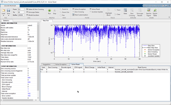
Profile the model using the Solver Profiler to find an appropriate step size for the candidate fixed-step simulations of the model. See Solver Profiler for information on how to launch and use the tool. For command-line usage, see solverprofiler.profileModel.

Note the maximum and average step sizes returned by the Solver Profiler.

             solver: 'ode45'
             tStart: 0
              tStop: 60
             absTol: 1.0000e-06
             relTol: 1.0000e-04
               hMax: 0.1000
           hAverage: 0.0447
              steps: 1342
        profileTime: 0.0665
           zcNumber: 0
        resetNumber: 600
     jacobianNumber: 0
    exceptionNumber: 193

Run Fixed-Step Simulations of the Model

Once you obtain the results of the variable-step simulation of the model, simulate it using one or more of the fixed-step solvers. In this example, the model is simulated using all the non-stiff fixed-step solvers: ode1, ode2, ode3, ode4, ode5, and ode8. You can also select a specific solver from the Solver dropdown in the Model Configuration Parameters to run against the variable-step baseline.

Considerations for Selecting a Fixed Step Size

The optimal step size for a fixed-step simulation of your model strikes a balance between speed and accuracy, given constraints such as code-generation objectives, physics or dynamics of the model, and modeling patterns used. For example, code generation would dictate the step size must be greater than or equal to the clock speed of the processor (the reciprocal of the CPU frequency). For pure simulation objectives, the step size must be less than the discrete sample times specified by individual blocks in the model. For models with periodic signals, the step size must be such that the signal is sampled at twice its highest frequency; this is known as the Nyquist frequency.

For this specific example, set the fixed-step size of the solver to 0.1 (the maximum step size detected by the Solver Profiler). This takes into account the discrete sample time 0.1 of the Dryden Wind-Gust block, as well as the periodic nature of the stick movements and the aircraft response.

Make sure that the model states, outputs, and simulation time are enabled for logging and that the logging format is set to Dataset in the Model Configuration Parameters.

Simulate the model by selecting any one or all the non-stiff fixed-step solvers from the Solver dropdown of the Model Configuration Parameters when the solver Type is set to Fixed-step.

A Simulink.sdi.Run object is created for the fixed-step solver simulation(s) and stored in the fsRuns struct in the base workspace.

Compare Fixed-Step Simulations with the Variable-Step Baseline

Use the Simulation Data Inspector to visualize and inspect logged signals in your model. You can also compare signals across simulations, or runs, using the Compare feature. For more information on using the Simulation Data Inspector, see Simulation Data Inspector. For more information on how to compare simulations using the Simulation Data Inspector, see Compare Simulation Data.

To compare signals, switch to the Compare tab in the Simulation Data Inspector. Set the Baseline run to the variable-step simulation and select a fixed-step simulation from the Compare to dropdown. Set the Global Abs Tolerance, Global Rel Tolerance, and Global Time Tolerance based on your requirements.

For this example, Global Abs Tolerance is set to 0.065, Global Rel Tolerance is set to 0.005, and Global Time Tolerance is set to 0.1.

The comparison plots display the results for the lowest order fixed-step solver simulation where all signals fell within tolerance, when compared to the baseline variable-step simulation. For the selected solver, comparison results of a few of the signals are plotted below.

The lowest order with all signals within tolerance is determined to be ode4. Consider the results for the ode1 fixed-step solver, where the comparison results showed 11 signals out of tolerance. Observe that there are 11 signals out of tolerance when the signal comparison parameters are set as:

• Signal Abs Tolerance: 0.065

• Signal Rel Tolerance: 0.065

• Signal Time Tolerance: 0.1