Main Content

Load Flow Analyzer

Perform positive-sequence load flow or unbalanced load flow and initialize models containing load flow blocks

Since R2021a

Description

The Load Flow Analyzer app uses the power_loadflow function and relies on the Newton-Raphson method to provide a robust and fast convergence solution.

The Load Flow Analyzer app allows you to perform two types of load flows:

  • Positive-sequence load flow applied to a three-phase system. Positive-sequence voltages and active power (P) and reactive power (Q) flows are computed at each three-phase bus.

  • Unbalanced load flow applied to a mix of three-phase, two-phase, and single-phase systems. Individual phase voltage and PQ flow are computed for each phase.

To solve a load flow, you need to determine these four quantities at each bus:

  • The net active power P and reactive power Q injected into the bus

  • The voltage magnitude V and angle Vangle of bus positive-sequence voltage (positive-sequence voltage or phase voltage)

Before solving the load flow, two of the above quantities are known at every bus and the other two are to be determined. Therefore, the following bus types are used:

  • PV bus — For this type of bus, specify P and V. This is a generation bus where a generator, such as a voltage source or three-phase synchronous machine, is connected. The active power P is generated and the generator terminal voltage V is imposed. The load flow solution returns the machine reactive power Q that is required to maintain the reference voltage magnitude V, and the reference voltage angle Vangle.

  • PQ bus — At this bus, the specified active power P and reactive power Q are either injected into the bus (generation PQ bus) or absorbed by a load connected at that bus. The load flow solution returns the bus voltage magnitude V and angle Vangle.

  • Swing bus — This bus imposes the voltage magnitude V and angle Vangle. The load flow solution returns the active power P and reactive power Q that is generated or absorbed at that bus in order to balance generated power, loads, and losses. At least one bus in the model must be defined as a swing bus, but usually a single swing bus is required unless you have isolated networks. For a positive-sequence load flow, you typically select one synchronous machine or voltage source as a swing bus. For an unbalanced load flow, you can select the three phases of a Three-Phase Voltage Source block or single-phase AC Voltage Source blocks as swing buses.

Use the Load Flow Bus block to define the buses in your model.

If you perform a positive-sequence load flow, you connect a Load Flow Bus block with the Connectors parameter specified as single to any phase (A, B, or C) of every load flow block in the model. When several load flow blocks are connected together at the same nodes, only one Load Flow Bus block is required to identify the bus.

If you perform an unbalanced load flow, you connect a Load Flow Bus block to all phases of every load flow block in the model. Depending on the number of phases, you need to specify the Connectors parameter by selecting either three connectors (ABC), two connectors (AB, AC, or BC) or a single connector (A, B, or C). When several load flow blocks are connected together at the same nodes, only one Load Flow Bus block is required to identify the bus. In the load flow report, each bus is identified by its Bus identification parameter followed by _a, _b, or _c.

Load Flow Blocks for Positive-Sequence Load Flow

Load flow blocks are Simscape™ Electrical™ Specialized Power Systems blocks in which you can specify active power (P) and reactive power (Q) to solve the positive-sequence load flow. They are:

  • Asynchronous Machine

  • Simplified Synchronous Machine

  • Synchronous Machine

  • Three-Phase Dynamic Load

  • Three-Phase Parallel RLC Load

  • Three-Phase Series RLC Load

  • Three-Phase Programmable Voltage Source

  • Three-Phase Source

You specify P and Q in the Load Flow tab of the block dialog boxes.

Load Flow Parameters of Three-Phase Sources and Synchronous Machines

The Three-Phase Source and Synchronous Machine blocks allow you to control the generated or absorbed powers P and Q and the positive-sequence terminal voltage. You can set Generator type to swing, PV, or PQ.

Load Flow Parameters of Asynchronous Machine Blocks

The Asynchronous Machine blocks require you to specify the mechanical power Pmec at the machine shaft.

Load Flow Parameters of the RLC Load Blocks

For the Three Phase RLC Load block, you can specify Load type as constant Z (impedance), constant PQ (power), or constant I (current).

Load Flow Parameters of Dynamic Load Blocks

The Three-Phase Dynamic Load block dialog box does not have a Load Flow tab. The load is always considered as a constant PQ load. P and Q are the initial active and reactive power Po, Qo that you specify by using the Active and reactive power at initial voltage [Po(W) Qo(var)] parameter. The Initial positive-sequence voltage Vo [Mag(pu) Phase (deg.)] parameter (Mag and Phase) updates according to the load flow solution.

Load Flow Blocks for Unbalanced Load Flow

Load flow blocks are Simscape Electrical Specialized Power Systems blocks in which you can specify active power (P) and reactive power (Q) to solve the load flow at each phase of every bus. They are:

  • AC Voltage Source

  • Asynchronous Machine

  • Parallel RLC Load

  • Series RLC Load

  • Synchronous Machine

  • Three-Phase Dynamic Load

  • Three-Phase Parallel RLC Load

  • Three-Phase Series RLC Load

  • Three-Phase Source

You specify P and Q in the Load Flow tab of the block dialog boxes.

Load Flow Parameters of Single-Phase and Three-Phase Sources

The single-phase AC Voltage Source block allows you to control the generated or absorbed powers P and Q and the terminal voltage. The Three-Phase Source block allows you to control the generated or absorbed powers P and Q and the terminal voltages for each phase (A, B, and C). For these two blocks, you can set Generator type to swing, PV, or PQ.

Load Flow Parameters of Synchronous Machine

The Three-Phase Synchronous Machine block allows you to control generated or absorbed powers P and Q (total of phases A, B, and C) and its positive-sequence terminal voltage. You can set Generator type to PV or PQ.

Load Flow Parameters of Asynchronous Machine Blocks

The Asynchronous Machine blocks require you to specify the mechanical power Pmec developed in positive-sequence at the machine shaft.

Load Flow Parameters of the RLC Load Blocks

You can specify the Load type parameter for the single-phase and three-phase RLC Load blocks as constant Z (impedance), constant PQ (power), or constant I (current). You can connect single-phase loads phase-to-ground or phase-to-phase. You can connect three-phase loads connected in Wye (grounded or floating) or delta.

Load Flow Parameters of Dynamic Load Blocks

The Three-Phase Dynamic Load block dialog box does not have a Load Flow tab. The load is always considered as a constant PQ load. P and Q are the initial active and reactive power Po, Qo that you specify by using the Active and reactive power at initial voltage [Po(W) Qo(var)] parameter. The Initial positive-sequence voltage Vo [Mag(pu) Phase (deg.)] parameter (Mag and Phase) updates according to the load flow solution.

Load Flow Analyzer app

Open the Load Flow Analyzer App

  • MATLAB® command prompt: Enter powerLoadFlow

  • powergui Block Parameters dialog box: On the Tools tab, click Load Flow Analyzer.

  • To perform a load flow analysis and initialize your model so that it starts in steady state:

    1. Define the model buses using Load Flow Bus blocks.

    2. Specify the load flow parameters of all blocks that have load flow parameters. These blocks are referred to as load flow blocks.

    3. Solve the load flow and interactively modify the load flow parameters until a satisfactory solution is obtained.

    4. Save the load flow parameters and machine initial conditions in the model.
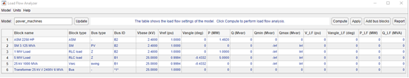
Examples

Positive-Sequence Load Flow

In the Command window, type power_LFnetwork_5bus to open a model containing five Load Flow Bus blocks and six load flow blocks.

The Load Flow Bus blocks are shown in orange and the load flow blocks are shown in yellow.

The Load Flow Bus blocks specify the bus base voltages (nominal phase-to-phase rms voltage). They also specify the voltage at PV buses or the voltage and angle of the swing buses. Once the load flow is solved, the Load Flow Bus block displays the bus positive-sequence voltage magnitude and phase angle as block annotations.

The bus type (PV, PQ, or swing) is determined by the load flow blocks connected to the bus. If you have several load flow blocks with different types (specified in the Generator type parameter or in the Load type parameter) connected to the same bus, the Load Flow tool determines the resulting bus type (swing, PQ, or PV).

In the power_LFnetwork_5bus example, the bus types are determined as follows:

BusLoad Flow BlocksResulting Bus Type

B120

120 kV Three-Phase Source
- Generator type = swing

swing
V=1.02 p.u. 0 deg.


Specify the voltage and angle in the B120 Load Flow Bus block.

B13.8

13.8 kV 150 MVA Synchronous Machine
- Generator type = PV

3 MW 2 Mvar RLC Load
- Load type = constant PQ

PV
P = 117 MW
V = 0.98 pu


Specify the voltage in the B13.8 Load Flow Bus block.

B25_1

10 MW, 3 Mvar Dynamic Load
- Implicit load type = constant PQ

PQ
P = –10 MW
Q = –3 Mvar

B25_2

No load flow blocks

PQ
P = 0 MW
Q = 0 Mvar

B575

Asynchronous generator 9 MW
1.2 Mvar RLC Load
- Load type = constant Z

PQ
P = 0 MW
Q = 0 Mvar


Constant Z load is included in the Ybus admittance matrix.

Some restrictions apply when you connect several source blocks and synchronous machines at the same bus:

  • Two swing generators cannot be connected in parallel.

  • A swing generator cannot be connected in parallel with a PV ideal voltage source.

  • When a swing voltage source with RL impedance is connected to a PV generator, the swing bus is automatically moved to the ideal voltage source connection node, behind the RL source impedance.

  • Only one PV generator with finite Q limits can be connected at a generation bus. However, you may have other PQ generators and loads connected on the same bus.

For more information on how to use the Load Flow Bus block in your model, see the Load Flow Bus page.

Using the Load Flow Tool to Perform Load Flow Analysis

Once you have entered the load flow parameters in the Load Flow Bus blocks and in the various load flow blocks, open the Load Flow Analyzer by clicking the Load Flow Analyzer button of the powergui block. The tool displays a summary of the load flow data of the model. The table below shows the data found in the power_LFnetwork_5bus model.

Note that the table contains seven lines, but there are only six load flow blocks in the model. This is because the bus B25_2 is not connected to any load flow block. Line 5 is added in the table for that particular bus, so that you can see all buses listed together with their bus voltages. This bus will be considered in the load flow analysis as a PQ bus with zero P and Q.

The Block name column identifies the block type. The Block type column displays the bus type of the load flow blocks. The next four columns give the bus identification label, the bus base voltage, the reference voltage (in pu of base voltage), and the voltage angle of the load flow bus where the block is connected. The following columns are the P and Q values specified in the Load Flow tab of the blocks.

The last four columns display the current load flow solution. Because the load flow has not been performed, the columns display zero values.

The load flow parameters in the Preferences tab of the powergui block are used to build the Ybus network admittance matrix and to solve the load flow. The base power is used to specify units of the normalized Ybus matrix in pu/Pbase and bus base voltages. The power_LFnetwork_5bus model contains five buses; consequently, the Ybus matrix will be a 5-by-5 complex matrix evaluated at the frequency specified by the Frequency (Hz) parameter.

The load flow algorithm uses an iterative solution based on the Newton-Raphson method. The Max iterations parameter defines the maximum number of iterations. The load flow algorithm will iterate until the P and Q mismatch at each bus is lower than the PQ tolerance parameter (in pu/Pbase). The power mismatch is defined as the difference between the net power injected into the bus by generators and PQ loads and the power transmitted on all links leaving that bus.

To avoid a badly conditioned Ybus matrix, you should select a Base power parameter value in the range of nominal powers and loads connected to the network. For a transmission network with voltages ranging from 120 kV to 765 kV, a 100 MVA base is usually selected. For a distribution network or for a small plant consisting of generators, motors, and loads that have a nominal power in the range of hundreds of kilowatts, a 1 MVA power base is better adapted.

To solve the load flow, click the Compute button. The load flow solution is displayed in the last five columns of the table.

To display the load flow report showing power flowing at each bus, click the Report button. Save this report in a file by specifying the file name at the prompt.

The report displays the summary of active and reactive powers, including the total PQ sharing between generators (SM- and Vsrc-type blocks), PQ loads (PQ-type RLC loads and DYN loads), shunt constant Z loads (Z-type RLC loads and magnetizing branches of transformers), and asynchronous machine loads (ASM):

The Load Flow converged in 2 iterations !        
                                                 
SUMMARY for subnetwork No 1                      
                                                 
Total generation :    P=  5.61 MW   Q= 25.51 Mvar
Total PQ load :       P= 13.00 MW   Q=  5.00 Mvar
Total Zshunt load :   P=  0.68 MW   Q= -0.51 Mvar
Total ASM load :      P= -8.90 MW   Q=  4.38 Mvar
Total losses :        P=  0.83 MW   Q= 16.64 Mvar

The Total losses line represents the difference between generation and loads (PQ type + Z type +ASM) and represents series losses. After this summary, a voltage and power report is presented for each bus:

1 : B120  V= 1.020 pu/120kV 0.00 deg  ; Swing bus 
        Generation : P= -114.39 MW Q=   62.76 Mvar
        PQ_load    : P=    0.00 MW Q=    0.00 Mvar
        Z_shunt    : P=    0.25 MW Q=    0.23 Mvar
   -->  B13.8      : P= -116.47 MW Q=   53.89 Mvar
   -->  B25_1      : P=    1.84 MW Q=    8.63 Mvar
                                                  
2 : B13.8  V= 0.980 pu/13.8kV -23.81 deg          
        Generation : P=  120.00 MW Q=  -37.25 Mvar
        PQ_load    : P=    3.00 MW Q=    2.00 Mvar
        Z_shunt    : P=    0.17 MW Q=    0.17 Mvar
   -->  B120       : P=  116.83 MW Q=  -39.42 Mvar
                                                  
3 : B25_1  V= 0.998 pu/25kV -30.22 deg            
        Generation : P=    0.00 MW Q=    0.00 Mvar
        PQ_load    : P=   10.00 MW Q=    3.00 Mvar
        Z_shunt    : P=    0.25 MW Q=    0.21 Mvar
   -->  B120       : P=   -1.83 MW Q=   -8.44 Mvar
   -->  B25_2      : P=   -8.41 MW Q=    5.23 Mvar
                                                  
4 : B25_2  V= 0.967 pu/25kV -20.85 deg            
        Generation : P=    0.00 MW Q=    0.00 Mvar
        PQ_load    : P=   -0.00 MW Q=   -0.00 Mvar
        Z_shunt    : P=    0.01 MW Q=   -0.03 Mvar
   -->  B25_1      : P=    8.87 MW Q=   -3.67 Mvar
   -->  B575       : P=   -8.88 MW Q=    3.70 Mvar
                                                  
5 : B575  V= 0.953 pu/0.575kV -18.51 deg          
        Generation : P=    0.00 MW Q=    0.00 Mvar
        PQ_load    : P=   -0.00 MW Q=   -0.00 Mvar
        Z_shunt    : P=    0.01 MW Q=   -1.09 Mvar
   -->  ASM        : P=   -8.90 MW Q=    4.38 Mvar
   -->  B25_2      : P=    8.89 MW Q=   -3.29 Mvar

For every bus, the bus voltage and angle are listed on the first line. The next three lines give the PQ generated at the bus (all SM and voltage sources), the PQ absorbed by the PQ type loads, and the PQ absorbed by the Z-type loads.

The last lines, preceded by an arrow (-->), list the PQ transmitted to neighbor buses connected through lines, series impedances, and transformers, as well power absorbed by ASM.

Apply the Load Flow Solution to Your Model

When performing a load flow analysis, you may need to iterate on P, Q, and V values until you find satisfactory voltages at all buses. This may require, for example, changing generated power, load powers, or reactive shunt compensation.

To change the load flow setup, you need to edit the parameters of the load flow blocks and the Load Flow Bus blocks. Then click the Update button to refresh the load flow data displayed by the table in the Load Flow Analyzer. The previous load flow solution is then deleted from the table. Click the Compute button to obtain a new load flow solution that corresponds to the changes you made.

Once you have obtained a satisfactory load flow, update the model initial conditions according to the load flow solution. Click the Apply to Model button to initialize the machine blocks of the model, and as the initial conditions of regulators connected to the machines.

Open the Three-Phase Parallel RLC Load block connected at the B13.8 bus. Because the Load type specified in the Load Flow tab is constant PQ, the nominal voltage of this block has been changed to the corresponding bus voltage of 0.98 pu. The Nominal phase-to-phase voltage Vn (Vrms) parameter is set to (13800)*0.98.

Open the Three-Phase Dynamic Load block connected at the B25_1bus. The Initial positive-sequence voltage Vo [Mag(pu) Phase (deg.) is set to [0.998241 -30.2228].

Note that the voltage magnitudes and angles obtained at each bus are written as block annotations under the Load Flow Bus blocks.

Open the Scope block and start the simulation.

The Three-Phase Fault block applies a six-cycle fault at the B120 bus.

Observe the waveforms of the SM active power, SM and ASM speeds, and PQ of DYN load, and notice that simulation starts in steady state.

Example of Unbalanced Load Flow

At the command prompt, enter power_13NodeTestFeeder to open a model containing 12 Load Flow Bus blocks and 13 load flow blocks. This model is a benchmark network taken from the Radial Distribution Test Feeder in the Distribution System Analysis Subcommittee Report by the Power Engineering Society in pages 908–912 written in 2001.

The original benchmark system contains 13 nodes. However, because the power_13NodeTestFeeder model does not include the regulating transformer, it contains only 12 nodes.

The Load Flow Bus blocks are shown in orange and the Load Flow blocks are shown in yellow.

The Load Flow Bus blocks specify the bus base voltages (nominal phase-to-ground rms voltage). They specify the voltage at PV buses or the voltage and angle of the swing buses. Once the load flow is solved, the Load Flow Bus block displays the bus voltage magnitude and phase angle as block annotations.

Note

By default, the block annotations are set in the Block Annotation tab of the Load Flow Bus block properties to display the phase A magnitude (<VLF> parameter) and the phase A angle (<angleLF> parameter). To display phase B magnitude and angle, specify <VLFb> and <angleLFb>, respectively. To display phase C magnitude and angle, specify <VLFc> and <angleLFc>, respectively.

You can also delete some block annotations. In the power_13NodeTestFeeder example, only the bus identification is displayed (<ID> parameter).

The bus type (PV, PQ, or swing) is determined by the load flow blocks connected to the bus. If you have several load flow blocks with different types (specified in the Generator type parameter or in the Load type parameter) connected to the same bus, the Load Flow tool determines the resulting bus type (swing, PQ, or PV). The table shows how the bus types are determined for some of the model buses of the power_13NodeTestFeeder example.

BusLoad Flow BlocksResulting Bus Type

632

4160 V swing
- Generator type = swing

632_a=swing V=1.0210 pu -2.49 deg.
632_b=swing V=1.042 pu -121.72 deg.
632_c=swing V=1.074 pu -121.72 deg.


Voltages and angles are specified in the ‘632’ Load Flow Bus block.

633

No load flow block

PQ
633_a -> P= 0 kW; Q = 0 kvar
633_b -> P= 0 kW; Q = 0 kvar
633_c -> P= 0 kW; Q = 0 kvar

634

634 Yg PQ load block
- Load type = constant PQ

PQ
634_a -> P= 160 kW; Q = 110 kvar
634_b -> P= 120 kW; Q = 90 kvar
634_c -> P= 120 kW; Q = 90 kvar

646

646_Z load block
- Load type = constant Z
- Load connection ‘bc’

PQ
646_bc -> P= 0 MW Q = 0 Mvar


Constant Z loads are included in the Ybus admittance matrix.

675

675 Yg PQ load
- Load type = constant PQ


675 Yg Z load
- Load type = constant Z

PQ
675_a -> P= 485 kW; Q = 190 kvar
675_b -> P= 68 kW; Q = 60 kvar
675_c -> P= 290 kW; Q = 212 kvar


Constant Z loads are included in the Ybus admittance matrix.

Some restrictions apply when you have several source blocks and synchronous machines connected to the same load flow bus:

  • You cannot connect two swing generators in parallel.

  • You cannot connect a swing generator in parallel with a PV ideal voltage source

  • You can connect only one PV generator with finite Q limits at a generation bus. However, you can have other PQ generators and loads connected on the same bus.

For more information on how to use the Load Flow Bus block in your model, see Load Flow Bus block.

Open the Load Flow Tool to Perform Load Flow Analysis

Open the Load Flow Analyzer by clicking the Load Flow Analyzer button in the powergui block. The tool displays a list of the individual single-phase buses (one bus per phase) found in the power_13NodeTestFeeder model. In the Load Flow Analyzer, the load flow has not yet been performed, so the V_LF (pu) and Vangle_LF (deg) columns display zero values.

The load flow parameters in the Preferences tab of the powergui block are used to build the Ybus network admittance matrix and to solve the load flow. The base power is used to specify units of the normalized Ybus matrix in pu/Pbase and bus base voltages. The power_13NodeTestFeeder model contains 29 single phase buses; consequently, the Ybus matrix is a 29-by-29 complex matrix evaluated at the frequency specified by the Frequency (Hz) parameter.

The load flow algorithm uses an iterative solution based on the Newton-Raphson method. The Max iterations parameter defines the maximum number of iterations. The load flow algorithm iterates until the P and Q mismatch at each bus is lower than the PQ tolerance parameter (in pu/Pbase). The power mismatch is defined as the difference between the net power injected into the bus by generators and PQ loads and the power transmitted on all links leaving that bus.

To avoid a badly conditioned Ybus matrix, select the Base power parameter value in the range of nominal powers and loads connected to the network. For a transmission network with voltages ranging from 120 kV to 765 kV, a 100 MVA base is usually selected. For a distribution network with loads that have a nominal power in the range of tens to hundreds of kVA, a 100 kVA to 1 MVA power base is better adapted.

To solve the load flow, click Compute. The bus voltages and angles appear in the V_LF (pu) and Vangle_LF (deg) columns of the table.

To display a load flow report that shows the power flow at each bus, click Report. Save this report in a file by specifying the file name at the prompt.

The report displays the summary of active and reactive powers, including the total PQ sharing between generators (SM- and Vsrc-type blocks), PQ loads (PQ-type RLC loads, dynamic loads, and asynchronous machine loads), and shunt constant Z loads (Z-type RLC loads and magnetizing branches of transformers):

SUMMARY for subnetwork No 1                                 
                                                            
  Total generation  : P=   3518.74 kW   Q=   1540.14 kvar   
  Total PQ load     : P=   3101.90 kW   Q=   1880.42 kvar   
  Total Zshunt load : P=    363.47 kW   Q=   -479.42 kvar   
  Total losses      : P=     53.36 kW   Q=    139.14 kvar   

The Total losses line represents the difference between generation and loads (PQ type + Zshunt type) and represents series losses. After this summary, a voltage and power report appears for each bus. For each phase of every bus, the bus voltage and angle are listed on the first line. The next three lines give the PQ generated at the bus (all SM and voltage sources), the PQ absorbed by the PQ type loads, and the PQ absorbed by the Z-type loads. The last lines, preceded by an arrow (–>), list the PQ power transmitted on all links leaving that bus.

The last column gives the positive-sequence bus voltage V1 (magnitude and angle, for three-phase buses only) and the sum of PQ powers for all phases (PQ generated by sources, PQ absorbed by loads, and PQ transmitted through transformers, lines, and series impedances). For example, you can verify that the total PQ load absorbed at bus 634 (P = 400 kW Q = 290 kvar) corresponds to the sum of active and reactive powers specified for phases A, B, and C in the load block.

Apply the Load Flow Solution to Your Model

When performing a load flow analysis, you might need to try different P, Q, and V values until you find satisfactory voltages at all buses. This can require, for example, changing generated power, load powers, or reactive shunt compensation.

To change the load flow setup, edit the parameters of the load flow blocks and of the Load Flow Bus blocks. Then click Update to refresh the load flow data displayed by the table. Click Compute to get a new load flow solution that corresponds to the changes you made.

Once you have a satisfactory load flow, update the model initial conditions according to the load flow solution. Click Apply to Model to initialize the PQ-type load blocks, the source block internal voltages, the machine blocks, and the initial conditions of associated regulators.

Open the Three-Phase Series RLC Load block connected at bus 632. Because the Load type specified in the Load Flow tab is constant PQ, the vector of Nominal phase-to-neutral voltages [Va Vb Vc] (Vrms) of this block has been changed to the corresponding bus voltages [1.021 1.042 1.0174]*2401.78 Vrms. Open the Three-Phase Source block connected at bus 632. The Line-to-neutral voltages [Va Vb Vc] (Vrms) parameter is also set to [1.021 1.042 1.0174]*2401.78 Vrms.

Open the Load Flow Results subsystem and start the simulation.

Observe voltage magnitudes and PQ powers on the Display blocks. These values correspond to values displayed in the load flow report.

Parameters

expand all

Name of model to perform load flow analysis on.

Click to get the latest changes in the model. Any previous load flow solution is cleared from the table.

Click to solve the load flow. The solution is displayed in the V_LF, Vangle_LF, P_LF, and Q_LF columns of the table. The load flow is performed at the frequency, base power, PQ tolerance, and max iterations specified in the Preferences tab of the powergui block.

Click to apply the load flow solution to the model.

Click to add Load Flow Bus blocks to the model. The Load Flow Analyzer app determines the load flow bus required for your model and adds Load Flow Bus blocks only in places where there is no Load Flow Bus block already connected.

Click to save a load flow report that shows the power flowing toward each bus. You can save the report in either Excel®or MATLAB format.

Version History

Introduced in R2021a

See Also

Functions