drawSamples

Class: HamiltonianSampler

Generate Markov chain using Hamiltonian Monte Carlo (HMC)

Syntax

chain = drawSamples(smp)
[chain,endpoint,accratio] = drawSamples(smp)
[chain,endpoint,accratio] = drawSamples(___,Name,Value)


Description

chain = drawSamples(smp) generates a Markov chain by drawing samples using the Hamiltonian Monte Carlo sampler smp.

[chain,endpoint,accratio] = drawSamples(smp) also returns the final state of the Markov chain in endpoint and the fraction of accepted proposals in accratio.

[chain,endpoint,accratio] = drawSamples(___,Name,Value) specifies additional options using one or more name-value pair arguments. Specify name-value pair arguments after all other input arguments.

Input Arguments

smp — Hamiltonian Monte Carlo sampler

HamiltonianSampler object

Hamiltonian Monte Carlo sampler, specified as a HamiltonianSampler object.

drawSamples draws samples from the target log probability density in smp.LogPDF. Use the hmcSampler function to create a sampler.

Name-Value Arguments

Specify optional pairs of arguments as Name1=Value1,...,NameN=ValueN, where Name is the argument name and Value is the corresponding value. Name-value arguments must appear after other arguments, but the order of the pairs does not matter.

Before R2021a, use commas to separate each name and value, and enclose Name in quotes.

Example: 'Burnin',500,'NumSamples',2000 generates a Markov chain by discarding 500 burn-in samples and then drawing 2000 samples.

Burnin — Number of burn-in samples to discard

1000 (default) | positive integer

Number of burn-in samples to discard from the beginning of the Markov chain, specified as a positive integer.

Example: 'Burnin',500

NumSamples — Number of samples to draw

1000 (default) | positive integer

Number of samples to draw from the Markov chain using the HMC sampler, specified as a positive integer.

The drawSamples method generates this number of samples after the burn-in period.

Example: 'NumSamples',2000

ThinSize — Markov chain thinning size

1 (default) | positive integer

Markov chain thinning size, specified as a positive integer.

Only one out of the 'ThinSize' number of samples are kept. The rest of the samples are discarded.

Example: 'ThinSize',5

StartPoint — Initial point to start sampling from

smp.StartPoint (default) | numeric column vector

Initial point to start sampling from, specified as a numeric column vector with the same number of elements as the StartPoint property of the sampler smp.

Example: 'StartPoint',randn(5,1)

VerbosityLevel — Verbosity level of Command Window output

0 (default) | positive integer

Verbosity level of Command Window output during sampling, specified as 0 or a positive integer.

With the value set to 0, drawSamples displays no details during sampling.

With the value set to a positive integer, drawSamples displays details of the sampling. To set the output frequency, use the 'NumPrint' name-value pair argument.

drawSamples displays the output as a table with these columns.

Heading	Description
ITER	Iteration number
LOG PDF	Log probability density at the current iteration
STEP SIZE	Leapfrog integration step size at the current iteration. If the step size is jittered, it can vary between iterations.
NUM STEPS	Number of leapfrog integration steps at the current iteration. If the number of steps is jittered, it can vary between iterations
ACC RATIO	Acceptance ratio, that is, the fraction of proposals that are accepted. The acceptance ratio is calculated from the beginning of sampling, including the burn-in period.
DIVERGENT	Number of times the sampler failed to generate a valid proposal due to the leapfrog iterations generating NaNs or Infs. When drawing samples, a nonzero value in the DIVERGENT column indicates that the chosen step size is above the stability threshold for some region of state space. To fix this issue, try to set the StepSize to a smaller value, draw new samples, and check that all values in the DIVERGENT column equal 0.

Example: 'VerbosityLevel',1

NumPrint — Verbose output frequency

100 (default) | positive integer

Verbose output frequency, specified as a positive integer.

If the 'VerbosityLevel' value is a positive integer, then drawSamples outputs sampling details every 'NumPrint' iterations.

Example: 'NumPrint',200

Output Arguments

chain — Markov chain generated using Hamiltonian Monte Carlo

numeric matrix

Markov chain generated using Hamiltonian Monte Carlo, returned as a numeric matrix.

Each row of chain is a sample, and each column represents one sampling variable.

endpoint — Final state of Markov chain

numeric column vector

Final state of the Markov chain, returned as a numeric column vector of the same length as smp.StartPoint.

accratio — Acceptance ratio

numeric scalar

Acceptance ratio of the Markov chain proposals, returned as a numeric scalar. The acceptance ratio is calculated from the beginning of sampling, including the burn-in period.

Examples

Draw Samples Using HMC Sampler

Create MCMC chains for a multivariate normal distribution using a Hamiltonian Monte Carlo (HMC) sampler.

Define the number of parameters to sample and their means.

NumParams = 100;
means = randn(NumParams,1);
standevs = 0.1;

First, save a function normalDistGrad on the MATLAB® path that returns the multivariate normal log probability density and its gradient (normalDistGrad is defined at the end of this example). Then, call the function with arguments to define the logpdf input argument to the hmcSampler function.

logpdf = @(theta)normalDistGrad(theta,means,standevs);

Choose a starting point of the sampler. Create the HMC sampler and tune its parameters.

startpoint = randn(NumParams,1);
smp = hmcSampler(logpdf,startpoint);
smp = tuneSampler(smp);

Draw samples from the posterior density, using a few independent chains. Choose different, randomly distributed starting points for each chain. Specify the number of burn-in samples to discard from the beginning of the Markov chain and the number of samples to generate after the burn-in. Set the 'VerbosityLevel' to print details during sampling for the first chain.

NumChains  = 4;
chains     = cell(NumChains,1);
Burnin     = 500;
NumSamples = 2000;
for c = 1:NumChains
    if c == 1
        showOutput = 1;
    else
        showOutput = 0;
    end
    chains{c} = drawSamples(smp,'Burnin',Burnin,'NumSamples',NumSamples,...
        'Start',randn(size(startpoint)),'VerbosityLevel',showOutput,'NumPrint',500);
end

|==================================================================================|
|   ITER   |    LOG PDF    |  STEP SIZE  |  NUM STEPS  |  ACC RATIO  |  DIVERGENT  |
|==================================================================================|
|      500 |  8.450463e+01 |   4.776e-01 |           5 |   9.060e-01 |           0 |
|     1000 |  8.034444e+01 |   4.776e-01 |           9 |   8.810e-01 |           0 |
|     1500 |  9.156276e+01 |   4.776e-01 |           2 |   8.867e-01 |           0 |
|     2000 |  8.027782e+01 |   2.817e-02 |           6 |   8.890e-01 |           0 |
|     2500 |  9.892440e+01 |   4.648e-01 |           2 |   8.904e-01 |           0 |

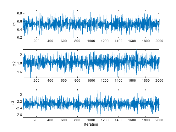
After obtaining a random sample, investigate issues such as convergence and mixing to determine whether the samples represent a reasonable set of random realizations from the target distribution. To examine the output, plot the trace plots of the samples for the first few variables using the first chain.

A number of burn-in samples have been removed to reduce the effect of the sampling starting point. Furthermore, the trace plots look like high-frequency noise, without any visible long-range correlation between the samples. This indicates that the chain is well mixed.

for p = 1:3
    subplot(3,1,p);
    plot(chains{1}(:,p));
    ylabel(smp.VariableNames(p))
    axis tight
end
xlabel('Iteration')

The normalDistGrad function returns the logarithm of the multivariate normal probability density with means in Mu and standard deviations in Sigma, specified as scalars or columns vectors the same length as the startpoint. The second output argument is the corresponding gradient.

function [lpdf,glpdf] = normalDistGrad(X,Mu,Sigma)
Z = (X - Mu)./Sigma;
lpdf = sum(-log(Sigma) - .5*log(2*pi) - .5*(Z.^2));
glpdf = -Z./Sigma;
end

Tips

• After creating an HMC sampler using the hmcSampler function, you can compute MAP (maximum-a-posteriori) point estimates, tune the sampler, draw samples, and check convergence diagnostics using the methods of the HamiltonianSampler class. For an example of this workflow, see Bayesian Linear Regression Using Hamiltonian Monte Carlo.

Version History

Introduced in R2017a