polyconf

R2026b

Polynomial confidence intervals

Syntax

Y = polyconf(p,X)

[Y,Delta] = polyconf(p,X,S)

[___] = polyconf(___,Name=Value)

Description

Y = polyconf(p,X) evaluates the polynomial p at each point in X. The argument p is a vector of length n+1 whose elements are the coefficients (in descending powers) of an nth-degree polynomial:

$$p(x)=p_1{x}^n+p_2{x}^{n-1}+\mathrm{...}+p_{n}x+p_{n+1}.$$

You can specify any vector for the coefficients in p, or calculate them using the polyfit function.

[Y,Delta] = polyconf(p,X,S) also returns the 95% prediction interval half-widths Delta for new observations at the values in X. To return Delta, you must specify S, which is an error estimation structure returned by the polyfit function.

[___] = polyconf(___,Name=Value) specifies options using one or more name-value arguments in addition to one of the previous syntaxes. For example, you can specify the confidence level for the confidence bounds.

Examples

Plot Polynomial Fit and Prediction Intervals

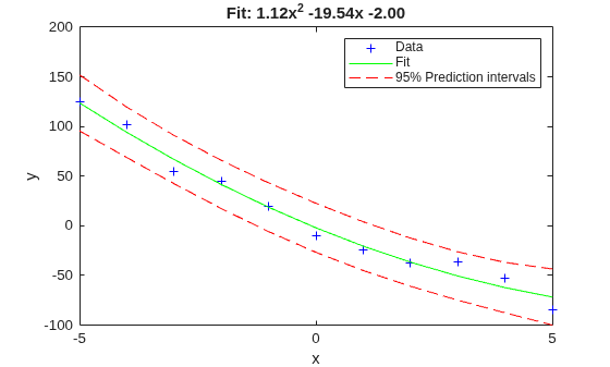
Fit a polynomial to a sample data set, and estimate the 95% prediction intervals and the roots of the fitted polynomial. Plot the data and the estimations, and display the fitted polynomial expression.

Generate sample data points (x,y) with a quadratic trend.

rng(0,"twister") % For reproducibility
x = -5:5;
y = x.^2 - 20*x - 3 + 5*randn(size(x));

Fit a second-degree polynomial to the data by using the polyfit function.

degree = 2;
[p,S] = polyfit(x,y,degree);

Estimate the 95% prediction intervals by using polyconf.

alpha = 0.05; % Significance level
[yfit,Delta] = polyconf(p,x,S,Alpha=alpha);

Plot the data, fitted polynomial, and prediction intervals, and display the fitted polynomial expression.

plot(x,y,"b+")
hold on
plot(x,yfit,"g-")
plot(x,yfit-Delta,"r--",x,yfit+Delta,"r--")
xlabel("x")
ylabel("y")
legend("Data","Fit","95% Prediction intervals")
title(["Fit: "+ sprintf("%.2fx^2 %+ .2fx %+ .2f",p(1),p(2),p(3))])
hold off

Find the roots of the polynomial p.

r = roots(p)

r = 2×1

   17.5152
   -0.1017

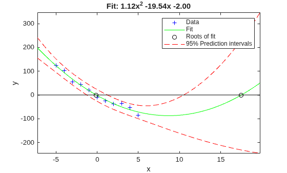
Because the roots are real values, you can plot them as well. Estimate the fitted values and prediction intervals for the x interval that includes the roots. Then, plot the roots and the estimations.

xmin = min([r(:);x(:)]);
xrange = range([r(:);x(:)]);
xExtended = linspace(xmin - 0.1*xrange, xmin + 1.1*xrange,1000);
[yfitExtended,deltaExtended] = polyconf(p,xExtended,S,Alpha=alpha);
plot(x,y,"b+")
hold on
plot(xExtended,yfitExtended,"g-")
plot(r,zeros(size(r)),"ko")
plot(xExtended,yfitExtended-deltaExtended,"r--")
plot(xExtended,yfitExtended+deltaExtended,"r--")
plot(xExtended,zeros(size(xExtended)),"k-")
xlabel("x")
ylabel("y")
legend("Data","Fit","Roots of fit","95% Prediction intervals")
title(["Fit: "+ sprintf("%.2fx^2 %+ .2fx %+ .2f",p(1),p(2),p(3))])
axis tight
hold off

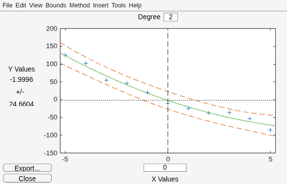
Alternatively, you can use the Polynomial Fitting Tool function for interactive polynomial fitting.

polytool(x,y,degree,alpha)

Input Arguments

p — Polynomial coefficients

numeric vector

Polynomial coefficients, specified as a numeric vector of length n+1 whose elements are the coefficients (in descending powers) of an nth-degree polynomial. For example, the vector [1 0 1] represents the polynomial $$x^2+1$$, and the vector [3.13 -2.21 5.99] represents the polynomial $$3.13x^2-2.21x+5.99$$.

Data Types: single | double

X — Query points

numeric matrix

Query points, specified as a numeric matrix. polyconf evaluates the polynomial p at the points in X and returns the corresponding function values in Y.

Data Types: single | double

S — Error estimation structure

structure

Error estimation structure, specified as a structure returned by the polyfit function. You must specify S to return the prediction interval half-widths, Delta. If you specify S, the dimension of the R field in the structure must equal the size of p.

Name-Value Arguments

Specify optional pairs of arguments as Name1=Value1,...,NameN=ValueN, where Name is the argument name and Value is the corresponding value. Name-value arguments must appear after other arguments, but the order of the pairs does not matter.

Example: polyconf(p,X,Alpha=0.01) specifies a confidence level of 99% for the confidence bounds.

Alpha — Significance level

0.05 (default) | numeric value in the range [0,1]

Significance level for the confidence interval, specified as a numeric value in the range [0,1]. The confidence level of y is equal to 100(1 – Alpha)%. Alpha is the probability that the confidence interval does not contain the true value.

Example: Alpha=0.01

Data Types: single | double

Mu — Centering and scaling values

two-element numeric vector

Centering and scaling values, specified as a two-element numeric vector. If you specify Mu, the function converts the query points in X to standardized z-scores using the mean value Mu(1) and standard deviation value Mu(2). To center the X values at zero with unit standard deviation, specify Mu=[mean(X),std(X)]. For more information about z-scores, see zscore.

Example: Mu=[1 1]

Data Types: single | double

PredOpt — Prediction interval to compute

"observation" (default) | "curve"

Prediction interval to compute, specified as "observation" or "curve". When the value is "observation", the function computes prediction intervals for new observations at the values in X. When the value is "curve", the function computes confidence intervals for the polynomial at the query points X.

For more information, see Prediction Intervals.

Example: PredOpt="curve"

Data Types: char | string

SimOpt — Indicator for specifying simultaneous bounds

"off" (default) | "on"

Indicator for specifying simultaneous bounds, specified as "on" or "off". Specify "off" to compute nonsimultaneous bounds, or "on" for simultaneous bounds.

For more information, see Prediction Intervals.

Example: SimOpt="on"

Data Types: char | string

Output Arguments

Y — Function values

numeric matrix

Function values, returned as a numeric matrix of the same size as the query points X. The matrix contains the results of evaluating the polynomial p at each point in X.

Delta — Confidence interval half-widths

numeric matrix

Confidence interval half-widths, returned as a numeric matrix. By default, Delta contains the half-widths for 95% prediction intervals for new observations at the values in X. You can compute the lower and upper bounds of the prediction intervals as Y – Delta and Y + Delta, respectively.

If the PredOpt value is "curve", Delta contains the half-widths for 95% confidence intervals for Y at the query points X.

More About

Prediction Intervals

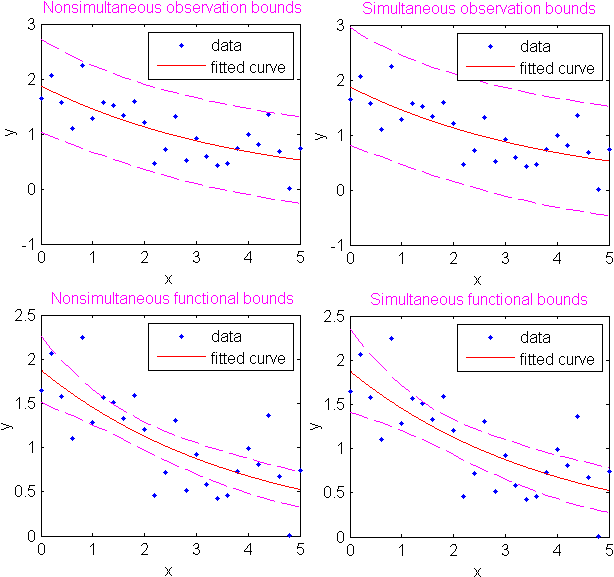
To better understand the PredOpt and SimOpt name-value arguments, consider the following functions:

• p(x) — Unknown mean function estimated by the fit

• l(x) — Lower confidence bound

• u(x) — Upper confidence bound

Suppose you have a new observation y_n+1 at x_n+1, so that

yn+1(xn+1) = p(xn+1) + εn+1

(1)

By default, the interval [l_n+1(x_n+1), u_n+1(x_n+1)] is a 95% confidence bound on y_n+1(x_n+1).

The following combinations of the PredOpt and SimOpt values allow you to specify other bounds.

SimOpt Value	PredOpt Value	Bounded Quantity
"off" (default)	"observation" (default)	yn+1(xn+1)
"off"	"curve"	p(xn+1)
"on"	"observation"	yn+1(x) for all x
"on"	"curve"	p(x) for all x

In general, "observation" (prediction) intervals are wider than "curve" (confidence) intervals, due to the additional uncertainty of predicting a new response value (the curve plus random errors). Likewise, simultaneous intervals are wider than nonsimultaneous intervals, due to the additional uncertainty of bounding values for all predictor values of x.

Version History

Introduced before R2006a