Visualize Wind Speed as a Function of Ambient Temperature and Pressure
This example shows how to visualize the variation of wind speed as a function of ambient air temperature and pressure using Curve Fitting Toolbox™. You read ThingSpeak™ data from a weather station and then use a 3D plot to visualize the data and the fit.
Read Data from the Weather Station ThingSpeak Channel
ThingSpeak channel 12397 contains data from the MathWorks weather station, located in Natick, Massachusetts. The data is collected once a minute. Fields 2, 4, and 6 contain wind speed, temperature, and air pressure data, respectively.
% Read the data using the |thingSpeakRead| function from channel 12397 on a particular week. For example, the week of May 1, 2018.
startDate = datetime('May 1, 2018 0:0:0');
endDate = datetime('May 8, 2018 0:0:0');
data = thingSpeakRead(12397,'daterange',[startDate endDate],'Fields',[2 4 6],'outputFormat','table');
Fit a Surface to the Data
Changes in both air pressure and temperature affect wind speed. Assume that the variation in wind speed is explained by a second degree polynomial in ambient temperature and pressure. Use the fit function to fit a quadratic surface.
fitObject = fit([data.TemperatureF,data.PressureHg],data.WindSpeedmph,'poly22');
Plot the Fitted Data
You can plot the fitted data to see if a quadratic surface fit captures the variation in wind speed.
plot(fitObject,[data.TemperatureF,data.PressureHg],data.WindSpeedmph);
xlabel('Ambient Temperature [^{\circ}F]');
ylabel('Ambient Air Pressure [inHg]');
zlabel('Wind Speed [mph]');
title('Wind Speed as a Function of Ambient Temperature and Pressure','FontSize',10);
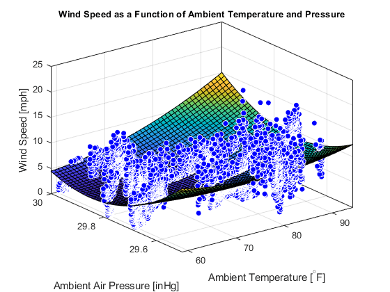
The quadratic fit appears to provide a good average for the fluctuating wind speed data. For this spring day, the wind speed is parabolic with rising pressure, but increses at larger temperatures.
See Also
Functions
fit(Curve Fitting Toolbox) |thingSpeakRead