Vehicle Steering Gain at Different Speeds
R2026bThis example shows how to sweep vehicle speed in the slowly increasing steering reference application and calculate the steering gain at each speed. The maneuver follows the constant speed, variable steer test defined in SAE J266.
During the maneuver, the driver:
Accelerates until vehicle hits a target velocity.
Maintains a target velocity.
Linearly increases the steering wheel angle from 0 degrees to a maximum angle.
Maintains the steering wheel angle for a specified time.
Linearly decreases the steering wheel angle from maximum angle to 0 degrees.
For more information about the reference application, see Slowly Increasing Steering Maneuver.
vdynblksIncreasingSteeringStart;
Run a Slowly Increasing Steering Maneuver
1. Open the Slowly Increasing Steer block. By default, the maneuver is set with these parameters:
Longitudinal speed setpoint — 50 mph
Handwheel rate — 13.5 deg/s
Maximum handwheel angle — 270 deg
2. In the Visualization subsystem, open the 3D Engine block. By default, the 3D Engine parameter is set to Disabled. Simulating models in the 3D visualization environment requires Simulink® 3D Animation™. For the 3D visualization engine platform requirements and hardware recommendations, see the Unreal Engine Simulation Environment Requirements and Limitations.
3. Run the maneuver with the default settings. As the simulation runs, view the vehicle information.
mdl = 'ISReferenceApplication';
sim(mdl);
### Searching for referenced models in model 'ISReferenceApplication'.
### Total of 3 models to build.
### Starting serial model build.
### Starting model reference simulation target build for: Driveline
### Successfully updated the model reference simulation target for: Driveline
### Starting model reference simulation target build for: PassVeh14DOF
### Successfully updated the model reference simulation target for: PassVeh14DOF
### Starting model reference simulation target build for: SiMappedEngineV
### Successfully updated the model reference simulation target for: SiMappedEngineV

Build Summary

Model reference simulation targets:

Model            Build Reason                                        Status                        Build Duration
=================================================================================================================
Driveline        Target (Driveline_msf.mexw64) did not exist.        Code generated and compiled.  0h 1m 10.856s
PassVeh14DOF     Target (PassVeh14DOF_msf.mexw64) did not exist.     Code generated and compiled.  0h 3m 17.948s
SiMappedEngineV  Target (SiMappedEngineV_msf.mexw64) did not exist.  Code generated and compiled.  0h 0m 37.083s

3 of 3 models built (0 models already up to date)
Build duration: 0h 5m 44.234s
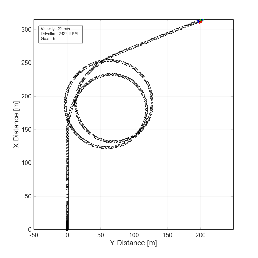
The Vehicle Position window displays the vehicle path (longitudinal distance versus lateral distance). The plot also shows the yaw rate and steering angle.
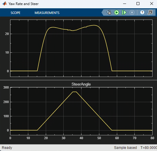
In the Visualization subsystem, open the Yaw Rate and Steer Scope block to display the yaw rate and steering angle versus time.
Sweep Vehicle Speed
Run the slowly increasing steering reference application with three different speed set points.
1. In the slowly increasing steering reference application model ISReferenceApplication, open the Slowly Increasing Steer block. The Longitudinal speed set point, velRef block parameter sets the vehicle speed. By default, the speed is 50 mph.
2. Enable signal logging for the velocity, lane, and ISO signals. You can use the Simulink® editor or, alternatively, these MATLAB® commands. Save the model.
Enable signal logging for the Slowly Increasing Steer Ref signal output port.
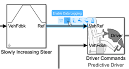
ph=get_param([mdl '/Slowly Increasing Steer'],'PortHandles');
set_param(ph.Outport(1),'DataLogging','on');
Enable signal logging for the Passenger Vehicle block output port signal.
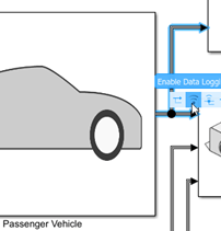
ph=get_param([mdl '/Passenger Vehicle'],'PortHandles');
set_param(ph.Outport(1),'DataLogging','on');
In the Visualization subsystem, enable signal logging for the ISO block.
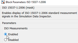
set_param([mdl '/Visualization/ISO 15037-1:2006'],'Measurement','Enable');
3. Define the speed set points to sweep. This example uses 45, 50, and 55 mph.
vmax = [45, 50, 55];
numExperiments = length(vmax);
4. Create an array of simulation inputs that set the Slowly Increasing Steer block parameter Longitudinal speed setpoint, velRef equal to vmax.
for idx = numExperiments:-1:1
    in(idx) = Simulink.SimulationInput(mdl);
    in(idx) = in(idx).setBlockParameter([mdl '/Slowly Increasing Steer'], ...
        'velRef', num2str(vmax(idx)));
end
5. Save the model and run the simulations.
save_system(mdl)
simout = parsim(in,'ShowSimulationManager','on');
[19-Jun-2026 16:19:24] Checking for availability of parallel pool...
[19-Jun-2026 16:19:24] Starting Simulink on parallel workers...
[19-Jun-2026 16:19:31] Loading project on parallel workers...
[19-Jun-2026 16:19:31] Configuring simulation cache folder on parallel workers...
[19-Jun-2026 16:19:31] Loading model on parallel workers...
[19-Jun-2026 16:20:42] Running simulations...
[19-Jun-2026 16:22:47] Completed 1 of 3 simulation runs
[19-Jun-2026 16:22:47] Received simulation output (size: 250.26 MB) for run 1 from parallel worker.
[19-Jun-2026 16:22:53] Completed 2 of 3 simulation runs
[19-Jun-2026 16:22:53] Received simulation output (size: 262.91 MB) for run 3 from parallel worker.
[19-Jun-2026 16:25:06] Completed 3 of 3 simulation runs
[19-Jun-2026 16:25:06] Received simulation output (size: 260.97 MB) for run 2 from parallel worker.
[19-Jun-2026 16:25:06] Cleaning up parallel workers...
Use Simulation Data Inspector to Analyze Results
Use the Simulation Data Inspector to examine the results. You can use the UI or, alternatively, command-line functions.
1. Open the Simulation Data Inspector. On the Simulink Toolstrip, on the Simulation tab, under Review Results, click Data Inspector.
In the Simulation Data Inspector, select Import.
In the Import dialog box, clear
logsout. Selectsimout(1),simout(2), andsimout(3). Select Import.
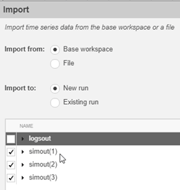
Use the Simulation Data Inspector to examine the results.
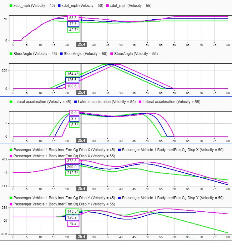
Use MATLAB commands to create SDI run objects, extract the longitudinal velocity, steering wheel angle, lateral acceleration, and vehicle position signals, and plot them. Assign distinct colors (green, blue, magenta) to distinguish the three speed conditions.
sigcolor=[0 1 0;0 0 1;1 0 1];
for idx = 1:numExperiments
    simoutRun(idx)=Simulink.sdi.Run.create;
    simoutRun(idx).Name=['Velocity = ', num2str(vmax(idx))];
    add(simoutRun(idx),'vars',simout(idx));
    msignal(idx)=getSignalsByName(simoutRun(idx), 'xdot_mph');
    msignal(idx).LineColor =sigcolor((idx),:);
    ssignal(idx)=getSignalsByName(simoutRun(idx), 'SteerAngle');
    ssignal(idx).LineColor =sigcolor((idx),:);
    asignal(idx)=getSignalsByName(simoutRun(idx), 'ay');
    asignal(idx).LineColor =sigcolor((idx),:);
    xsignal(idx)=getSignalsByName(simoutRun(idx), 'Passenger Vehicle:1.Body.InertFrm.Cg.Disp.X');
    xsignal(idx).LineColor =sigcolor((idx),:);
    ysignal(idx)=getSignalsByName(simoutRun(idx), 'Passenger Vehicle:1.Body.InertFrm.Cg.Disp.Y');
    ysignal(idx).LineColor =sigcolor((idx),:);
end
Simulink.sdi.view
Simulink.sdi.setSubPlotLayout(5,1);
for idx = 1:numExperiments
    plotOnSubPlot(msignal(idx),1,1,true);
    plotOnSubPlot(ssignal(idx),2,1,true);
    plotOnSubPlot(asignal(idx),3,1,true);
    plotOnSubPlot(xsignal(idx),4,1,true);
    plotOnSubPlot(ysignal(idx),5,1,true);
end
The results are similar to these plots, which indicate that the greatest lateral acceleration occurs when the vehicle velocity is 55 mph.
Further Analysis
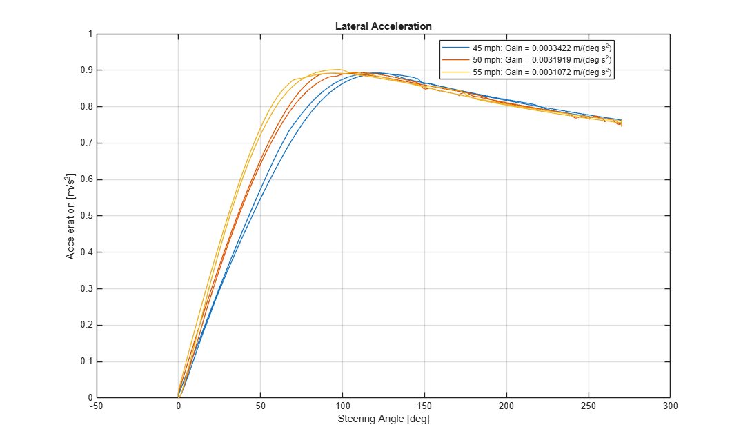
To understand the relationship between steering input and lateral response at each speed, extract the steering angle and lateral acceleration from the simulation output and compute the steering gain.
Extract the lateral acceleration and steering angle. Plot the data. The results are similar to this plot.
figure
for idx = 1:numExperiments
    log = get(simout(idx),'logsout');
    sa=log.get('SteerAngle').Values;
    ay=log.get('<ay>').Values;
    firstorderfit = polyfit(sa.Data,ay.Data,1);
    gain(idx)=firstorderfit(1);
    legend_labels{idx} = [num2str(vmax(idx)), ' mph: Gain = ', ...
        num2str(gain(idx)), ' m/(deg s^2)'];
    plot(sa.Data,ay.Data)
    hold on
end
legend(legend_labels, 'Location', 'best');
title('Lateral Acceleration')
xlabel('Steering Angle [deg]')
ylabel('Acceleration [m/s^2]')
grid on
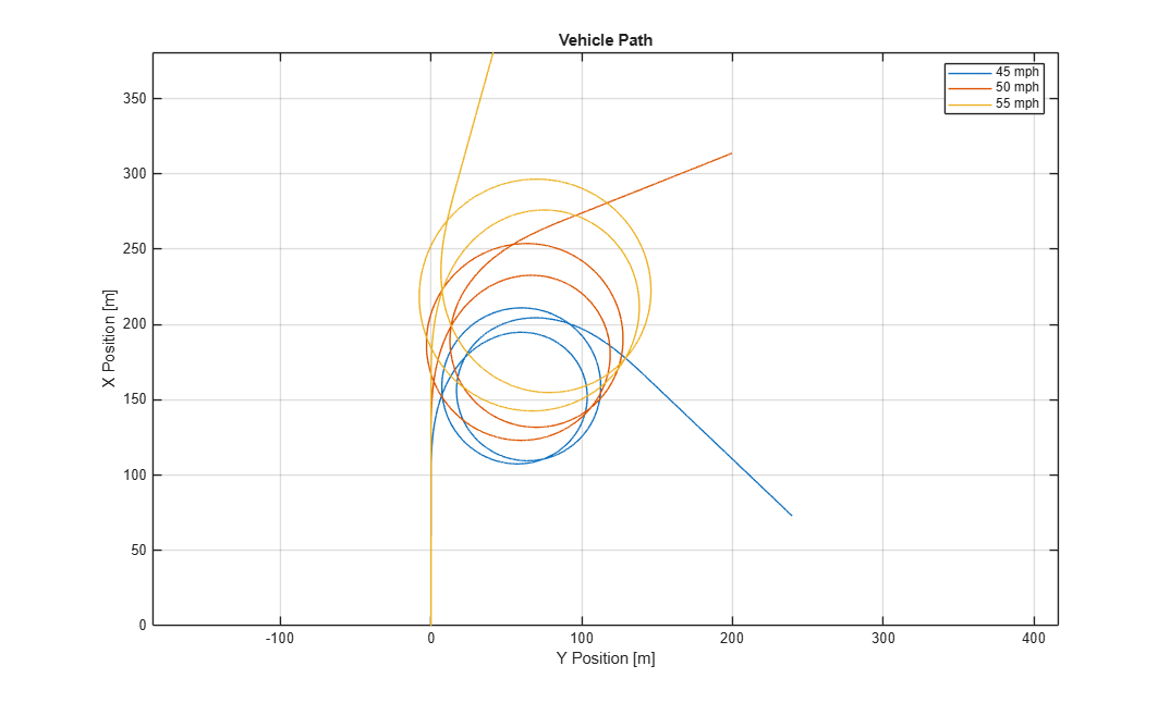
To visualize how the vehicle path changes with speed, plot the X-Y vehicle trajectory. The results are similar to this plot.
figure
for idx = 1:numExperiments
    xValues = getSignalsByName(simoutRun(idx), 'Passenger Vehicle:1.Body.InertFrm.Cg.Disp.X').Values;
    yValues = getSignalsByName(simoutRun(idx), 'Passenger Vehicle:1.Body.InertFrm.Cg.Disp.Y').Values;
    x = xValues.Data;
    y = yValues.Data;
    legend_labels{idx} = [num2str(vmax(idx)), ' mph'];
    axis('equal')
    plot(y,x)
    hold on
end
legend(legend_labels, 'Location', 'best');
title('Vehicle Path')
xlabel('Y Position [m]')
ylabel('X Position [m]')
grid on
References
[1] SAE J266. Steady-State Directional Control Test Procedures For Passenger Cars and Light Trucks. Warrendale, PA: SAE International, 1996.
See Also
Simulink.SimulationInput | Simulink.SimulationOutput | polyfit

