Flight Envelope Analysis for High-Altitude Fixed‑Wing Aircraft
R2026bThis example demonstrates how to evaluate the performance and maneuvering limits of a fixed‑wing aircraft intended for high‑altitude imaging missions. Flight‑envelope analysis evaluates whether early design assumptions support the mission profile. The example workflow generates several envelopes to examine sensitivity to altitude, structural limits, gust loading, and key aerodynamic parameters.
Define a baseline configuration.
Use flight envelopes to evaluate maneuvering capability and operational boundaries. When a maneuverability requirement is not met, an updated aircraft configuration is considered to demonstrate a typical conceptual‑design iteration loop.
Requirements and Aircraft Definition
The fixed-wing aircraft supports high-altitude imaging with these requirements:
Maximum Mach 0.78 above 10 km altitude
Maximum EAS 98 m/s below 10 km altitude
Maximum altitude of 18 km
Light to moderate atmospheric gust tolerance
Minimum turn radius ≤ 2.5 km at 15 km altitude
Adequate margins to stall, load‑factor limits, dynamic pressure constraints, and structural speed boundaries
A baseline aircraft configuration is represented using a struct. The mass and wing area are chosen for moderate wing loading, the CL limits represent a clean configuration with typical airfoil camber, and the load-factor limits reflect values used for comparable high-altitude aircraft.
cruiseAlt = 15000;    % m
[~, a, P, rho] = atmosisa(cruiseAlt);

%% Baseline aircraft configuration
ac.m       = 28000;     % kg
ac.S       = 186;       % m^2
ac.c       = 4.5;       % m (mean aerodynamic chord, reference)
ac.VneSL   = 98;        % m/s (EAS below 10km altitude)
ac.VneAlt  = correctairspeed(a * 0.78, a, P, 'TAS', 'EAS'); % m/s (EAS above 10km)
ac.Vcruise = correctairspeed(a * 0.7,  a, P, 'TAS', 'EAS'); % m/s (EAS)

ac.CLlim   = [-0.6, 1.2];    % clean configuration
ac.nLim    = [-1, 2.3];      % conceptual structural limits

ac.Gusts   = [5, 10, 15]; % m/s (light/moderate/occasionally rough during climb)
ac.Cla     = 5.4;         % 1/rad
ac.g       = 9.81;        % m/s^2

ac.Units       = "Metric";
ac.Atmosphere  = "ISA";
Plot Formatting Options
The flight envelope plotting functions support drawing the envelope boundary using BoundaryLine. Boundary lines help to clearly demarcate feasible and non-feasible areas of the envelope when presenting a single envelope. However, they can clutter the figure. For readability, this example enables "BoundaryLine","on" in figures where a single envelope is shown and disables it when multiple overlays might cause visual clutter.
These flight envelope plotting functions also support a Units option. This example uses metric units, but you can change the Units name-value argument to plot in English units, which can be more familiar when comparing against published aircraft performance data.
The following sections analyze flight envelopes to understand stall boundaries, maneuvering limits, gust sensitivity, and altitude‑dependent speed capability. We evaluate whether the baseline geometric and aerodynamic assumptions can meet the requirements. To illustrate typical conceptual‑design iteration, the example uses sensitivity cases.
Analyze Load Factor Envelope
Baseline Envelope
A Velocity Load‑Factor (V‑n) envelope shows structural and aerodynamic limits as a function of equivalent airspeed. At the conceptual stage, a sea‑level V‑n envelope provides an effective first check on achievable lift and associated load factor margins.
h0 = 0; % m
ax1 = velocityLoadFactorEnvelope( ...
    h0, ac.m, ac.S, ac.c, ac.VneSL, ac.CLlim, ac.nLim, ...
    "Cla", ac.Cla, ...
    "Gravity", ac.g, ...
    "Units", ac.Units, ...
    "BoundaryLine","on", ...
    "GustVelocities",[]);
title("Baseline Velocity–Load‑Factor Envelope (Sea Level)")
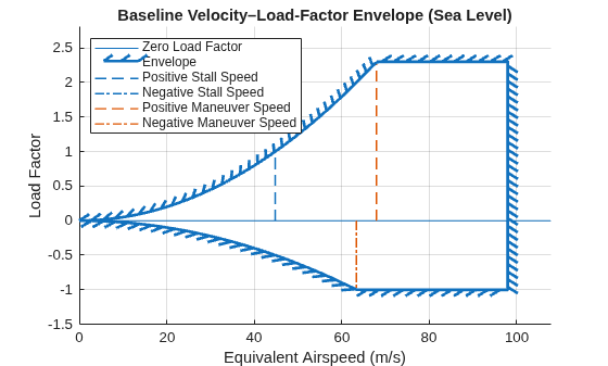
At low speeds, stall onset limits the maximum achievable load factor. At high speeds, structural load-factor limits and the never-exceed speed bound the envelope.
Gust Effects on Load Factor
Low altitude segments, such as climb, often encounter turbulence. Gusts can rapidly change the load factor, so structural margins must sufficiently account for gust-induced loads. Intersections between gust lines and the V-n envelope highlight where gusts push the aircraft toward or beyond structural limits.
h2000 = 2000; % m
f2 = figure("Position", [200 200 700 500]);
ax2 = axes(f2);
ax2 = velocityLoadFactorEnvelope(ax2, ...
    h2000, ac.m, ac.S, ac.c, ac.VneSL, ac.CLlim, ac.nLim, ...
    "Cla", ac.Cla, ...
    "Vcruise", ac.Vcruise, ...
    "GustVelocities", ac.Gusts, ...
    "Gravity", ac.g, ...
    "Units", ac.Units);
title("V–n Envelope with Gust Lines at 2000m")
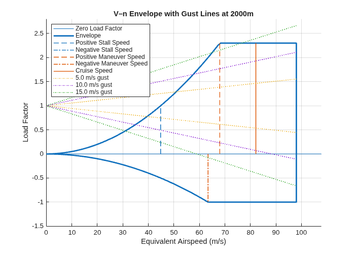
At 2000 m, gust-induced load factor increments become limiting at moderate-to-strong turbulence levels. The +15 m/s gust line exceeds the positive limit across most of the operational speed range, indicating that a 15 m/s upward gust exceeds structural load factor limits across most of the speed range shown. For comparison, the FAR Part 25 gust requirements define reference gusts at 2000 m altitude to be around 15.5 m/s.
Sensitivity Analysis
Early‑stage aircraft design carries uncertainty in both structural margins and weight estimates. To illustrate how these uncertainties affect maneuverability, the example generates a sensitivity case in which the aircraft mass is increased by 10% and the allowable load‑factor limits are reduced.
nLimReduced = [-0.8, 2];
f3 = figure("Position", [200 200 700 500]);
ax3 = axes(f3);
ax3 = velocityLoadFactorEnvelope(ax3, ...
    h2000, 1.1*ac.m, ac.S, ac.c, ac.VneSL, ac.CLlim, nLimReduced, ...
    "Cla", ac.Cla, ...
    "GustVelocities", ac.Gusts, ...
    "Gravity", ac.g, ...
    "Units", ac.Units);
title("V–n Envelope with Reduced Load‑Factor Limits (Design Sensitivity)")
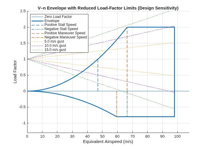
The combined effect of increased weight and reduced structural limits shrinks the maneuvering envelope, especially at mid‑to‑high speeds. The +15 m/s gust line now entirely exceeds the envelope and the +10 m/s gust line reaches the maximum load factor at speeds below the never-exceed speed, indicating that even a moderate upward gust over stresses the aircraft.
Overall, the sensitivity envelopes suggest that any combination of weight growth or reduced structural limits quickly degrades gust tolerance, and even modest gusts may require airspeed management at low altitude to avoid limit‑load boundaries.
Analyze Turn Rate Envelope
While the V–n diagram bounds permissible lift/load‑factor combinations, turning performance depends on how these limits interact with speed and altitude. We now examine the turn rate envelope.
The mission requires a minimum sustained turn radius of 2.5 km at 15 km altitude. A turn rate envelope shows the achievable turn rates and corresponding turn radii based on aerodynamic and load‑factor limits.
A turn rate envelope is first plotted at 5000 m as a low‑altitude reference, with radius and load‑factor guides.
[~, a5000, P5000, ~] = atmosisa(5000);
CLmax = ac.CLlim(2);
nMax  = ac.nLim(2);
vMax  = correctairspeed(ac.VneSL, a5000, P5000, 'EAS', 'TAS'); % TAS

ax4 = turnRateAirspeedEnvelope( ...
    CLmax, ac.S, ac.m, nMax, vMax, ...
    "Altitude", 5000, ...
    "Gamma", 0, ...
    "Radii", [1500 2500 4000], ...
    "LoadFactors", [1.2 1.4 1.8], ...
    "Gravity", ac.g, ...
    "Units", ac.Units, ...
    "BoundaryLine", "on", ...
    "AngleUnits","Degrees");
title("Turn Rate vs Airspeed at 5000m")
legend(Location="west")
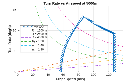
At low altitude, higher air density reduces stall speed, enabling higher load factors and greater turn performance. With increasing altitude, stall speed rises and air density decreases, degrading sustained turn performance.
[~, a15000, P15000, ~] = atmosisa(15000);
vMax = correctairspeed(ac.VneAlt, a15000, P15000, 'EAS', 'TAS'); % TAS
ax5 = turnRateAirspeedEnvelope( ...
    CLmax, ac.S, ac.m, nMax, vMax, ...
    "Altitude", cruiseAlt, "Gamma", 0, ...
    "Radii", [1500 2500 4000], ...
    "LoadFactors", [1.2 1.4 1.8], ...
    "Gravity", ac.g, ...
    "Units", ac.Units, ...
    "AngleUnits", "Degrees", ...
    "Atmosphere", ac.Atmosphere);
title("Turn‑Rate Envelope at Cruise Altitude (15000m)")
legend(Location="west")
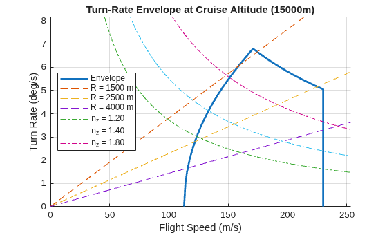
Even with identical structural speed limits, sustained turn capability degrades at high altitude. The 2.5 km radius lies near the envelope limit at high speeds, suggesting that either additional lift capability or relaxed maneuvering requirements might be needed.
Analyze Altitude and Airspeed Envelope
We now examine the altitude–airspeed envelope to see how stall, structural speed, dynamic pressure, and Mach constraints bound aircraft operation across altitude.
The baseline altitude–speed envelope shows how the stall boundary and structural speed limit bound the operable speed range across altitude.
hMax = 18000;

ax6 = altitudeSpeedEnvelope( ...
    ac.CLlim(2), hMax, vMax, ac.S, ac.m, ...
    "Units",ac.Units, ...
    "HMin",0, ...
    "Gravity",ac.g, ...
    "XAxis","TAS", ...
    "BoundaryLine","on");
title("Altitude–Airspeed Envelope (TAS)")
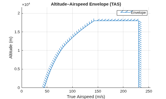
The TAS envelope alone is incomplete because it does not directly reflect other aerodynamic constraints. At high altitude, a Mach limit clips the right side and at low altitude, a dynamic pressure limit caps the high-speed boundary.
Qmax    = 5880;         % Pa; chosen to match earlier VneSL of 98 m/s
MachMax = 0.78;         % proxy for subsonic buffet and compressibility onset
MachLine  = [0.3 0.45 0.6 0.7];

ax7 = altitudeSpeedEnvelope( ...
    CLmax, hMax, vMax, ac.S, ac.m, ...
    "Units", ac.Units, ...
    "MachLines", MachLine, ...
    "MachMax", MachMax, ...
    "QMax", Qmax, ...
    "HMin", 0, ...
    "Gravity", ac.g, ...
    "XAxis", "TAS", ...
    "Atmosphere", ac.Atmosphere);
title("Altitude–Airspeed Envelope with QMax and Mach Lines (TAS View)")
legend(Location="northwest")
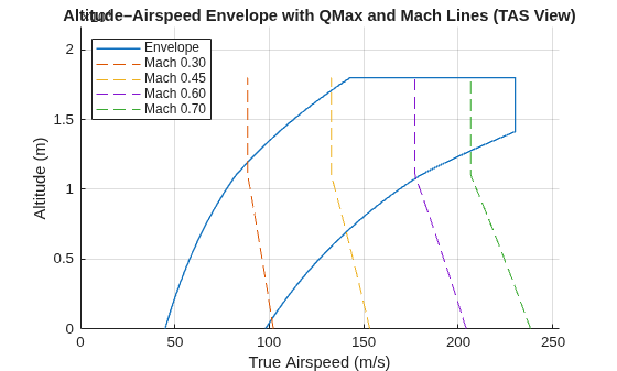
At low altitude, the dynamic pressure limit defines the right-hand boundary. At high altitude, the maximum Mach line truncates the speed range even when structural limits are otherwise permissive. A complementary EAS envelope removes altitude-dependent density effects from the x-axis, making stall and dynamic pressure limits appear as vertical boundaries.
ax8 = altitudeSpeedEnvelope( ...
    CLmax, hMax, vMax, ac.S, ac.m, ...
    "Units", ac.Units, ...
    "MachLines", MachLine, ...
    "MachMax", MachMax, ...
    "QMax", Qmax, ...
    "HMin", 0, ...
    "Gravity", ac.g, ...
    "XAxis", "EAS", ...
    "Atmosphere", ac.Atmosphere);
title("Altitude–Airspeed Envelope with QMax and Mach Lines (EAS View)")
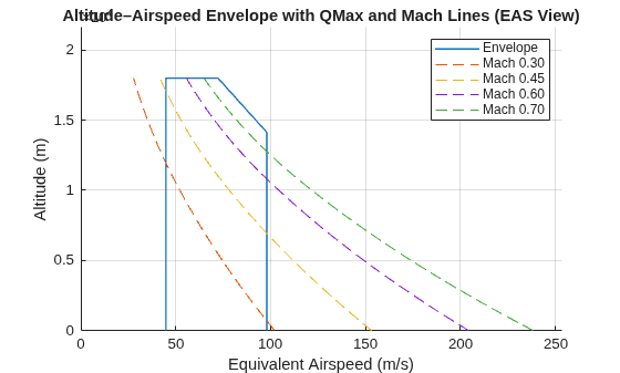
The constant dynamic pressure constraint is vertical in EAS, matching its structural meaning. In contrast, Mach limits remain slanted because they depend on true airspeed and temperature.
Summary
This example demonstrates a high‑subsonic flight envelope study where aerodynamics, structures, dynamic pressure limits, and compressibility shape the operable flight region.
Baseline V–n and turn rate envelopes define structural and aerodynamic bounds.
Gust‑line overlays identify rough‑air margins and potential exceedances.
Altitude–speed envelopes with Qmax and MachMax show how low‑altitude dynamic‑pressure and high‑altitude compressibility/buffet jointly limit the corridor.
At 15 km, the 2.5 km turn radius requirement can be assessed directly from the turn rate envelope, guiding trades between lift capability, structural limits, and speed constraints.
This workflow mirrors preliminary design practice for aircraft operating in the high‑subsonic regime, where Mach effects and dynamic pressure constraints are integral to the definition of feasible operating envelopes.
See Also
altitudeSpeedEnvelope | atmosisa | turnRateAirspeedEnvelope | velocityLoadFactorEnvelope

