dielectric
R2026bDielectric material to use as antenna substrate
Description
Dielectric material used as a substrate for antennas.
Creation
Description
creates a dielectric object with pre-defined materials from the dielectric
catalog. You can specify a single or multiple dielectric materials from the
catalog. Use this dielectric object as a substrate in antenna objects.d = dielectric(material)
creates a custom dielectric material based on the properties
specified using one or more name–value arguments. d = dielectric(PropertyName=Value)PropertyName is the
property name and Value is the corresponding value. You can specify
several name-value arguments in any order as
PropertyName1=Value1,...,PropertyNameN=ValueN. Properties that you do
not specify, retain their default values.
For example, d =
dielectric(Name="CustomDielectric",EpsilonR=4.5,LossTangent=0.02,Thickness=1e-3)
creates a custom dielectric material of 1mm. thickness with relative permittivity of 4.5,
and loss tangent of 0.02.
Input Arguments
Material from the dielectric catalog, specified as a single string for a single
material or comma separated strings for multiple materials. You can choose any
dielectric material with pre-defined properties from the dielectric
catalog. When you specify multiple dielectric materials,
dielectric object combines them into a single layer with a default
total thickness. You then specify the thickness of individual materials to use this
multi-material layer as an antenna substrate. You can also create an array of
dielectric materials.
Example:
dielectric("FR4") creates a single dielectric layer of FR4
material.
Example: dielectric("FR4","Teflon") creates a dielectric layer
made of FR4 and Teflon material.
Example: [dielectric("FR4")
dielectric("Teflon")] creates a 1-by-2
dielectric array of FR4 and Teflon materials.
Data Types: string
Properties
Name of the dielectric material, specified as a string for single material or a cell array of strings for multiple materials.
Example: "Taconic_TLC"
Example: {"FR4" "Teflon"}
Data Types: string
Relative permittivity of the dielectric material, specified as a positive scalar for a single dielectric material or a positive vector for multiple dielectric materials.
Example: 4.8000
Example: [4.8 6.5]
Data Types: double
Loss in the dielectric material, specified as a positive scalar for a single dielectric material or a positive vector for multiple dielectric materials.
Note
In the Antenna Toolbox™, the upper limit to loss tangent value is 0.03.
Example: 0.0260
Example: [0.026 0.028]
Data Types: double
Thickness of the dielectric material along z-axis, specified as a positive scalar or positive vector in meters. Specify scalar value for single dielectric material and vector value for multiple dielectric materials.
Example:
0.05
Example: [1e-3 2e-3]
Data Types: double
Analysis frequency for dispersion models, specified as a positive vector in Hz. For
the TableDriven model, specify Frequency as the
vector of frequency points at which you measured the dielectric properties. This vector
must have the same length as EpsilonR and
LossTangent, with each element corresponding to one measured data
point.
Example: 200e6
Data Types: double
Frequency dispersion model for dielectric material, specified as a string. The
default frequency model is Constant. Other supported frequency models
are as below:
Frequency independent:
ConstantFrequency dependent:
DjordjevicSarkar,MeanDjordjevicSarkar, andTableDriven.
The DjordjevicSarkar model uses extrapolation
techniques to predict properties of dielectric materials over a wide frequency range
from a single frequency point measurement. The MeanDjordjevicSarkar
model uses average value of the DjordjevicSarkar model over a
frequency range of interest to predict properties of dielectric materials. The
TableDriven model uses the dielectric material property values that
you specify at the corresponding frequency points. At each specified frequency point,
the model returns your tabulated data directly. The model applies a rational (causal)
fit only to interpolate between the specified frequency points and to extrapolate beyond
the specified frequency range. Use the frequency independent model for narrow band
applications. Use the frequency dependent models for wideband applications.
Note
The rational fit used for interpolation and extrapolation with the
TableDriven model requires an RF Toolbox™
license. The behavior of the TableDriven model depends on whether
you evaluate the material at a specified frequency point and on whether an RF Toolbox
license is available.
Example: "DjordjevicSarkar"
Data Types: string
Object Functions
getMaterialProperties | Calculate dielectric properties of material |
Examples
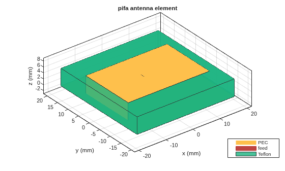
Use a Teflon dielectric material as a substrate for a PIFA antenna. View the antenna.
d = dielectric("Teflon")d =
dielectric with properties:
Name: 'Teflon'
EpsilonR: 2.1000
LossTangent: 2.0000e-04
Thickness: 0.0060
FrequencyModel: 'Constant'
For more materials see catalog
p = pifa(Height=0.0060,Substrate=d)
p =
pifa with properties:
Length: 0.0300
Width: 0.0200
Height: 0.0060
Substrate: [1×1 dielectric]
GroundPlaneLength: 0.0360
GroundPlaneWidth: 0.0360
PatchCenterOffset: [0 0]
ShortPinWidth: 0.0200
FeedOffset: [-0.0020 0]
Conductor: [1×1 metal]
Tilt: 0
TiltAxis: [1 0 0]
Load: [1×1 lumpedElement]
show(p)
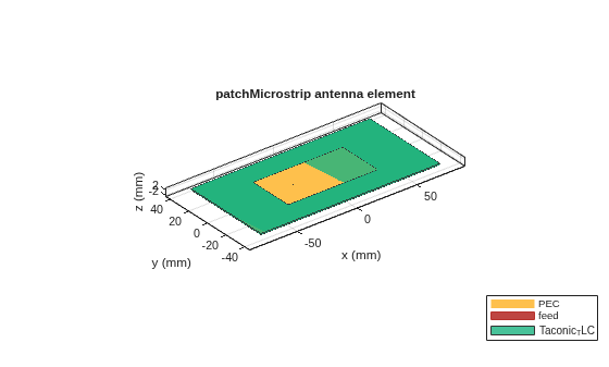
Create a patch microstrip antenna using a substrate with a relative permittivity of 2.70, a loss tangent of 0.002 and a thickness of 0.0008 m. View the antenna.
t = dielectric(Name="Taconic_TLC",EpsilonR=2.70,LossTangent=0.002,... Thickness=0.0008); p = patchMicrostrip(Height=0.0008,Substrate=t)
p =
patchMicrostrip with properties:
Length: 0.0750
Width: 0.0375
Height: 8.0000e-04
Substrate: [1×1 dielectric]
GroundPlaneLength: 0.1500
GroundPlaneWidth: 0.0750
PatchCenterOffset: [0 0]
FeedOffset: [-0.0187 0]
Conductor: [1×1 metal]
Tilt: 0
TiltAxis: [1 0 0]
Load: [1×1 lumpedElement]
show(p)
Create a microstrip patch antenna.
p = patchMicrostrip;
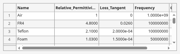
For property values of air and teflon dielectrics, refer Dielectric Catalog.
openDielectricCatalog
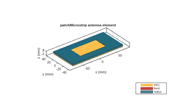
Use Teflon as a dielectric substrate. There is an air gap between the patch groundplane and the dielectric.
sub = dielectric(Name=["Air" "Teflon"],EpsilonR=[1 2.1],... Thickness=[0.002 0.004],LossTangent=[0 2e-04]);
Add the substrate to the patch antenna.
p.Substrate = sub; figure show(p)
Create a microstrip patch antenna.
p = patchMicrostrip;
For dielectric properties, use the Dielectric Catalog.
openDielectricCatalog
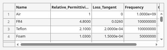
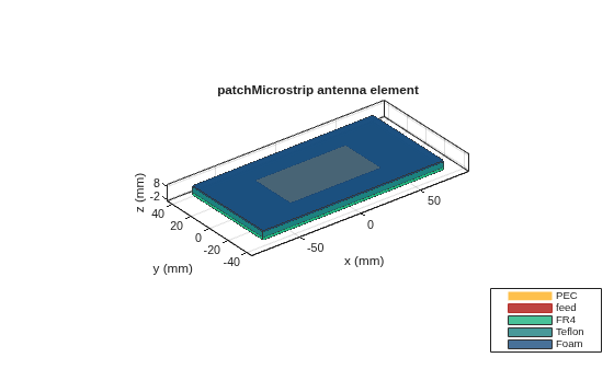
Use FR4, Teflon and Foam as the three layers of the substrate.
sub = dielectric(Name=["FR4" "Teflon" "Foam"],EpsilonR=... [4.80 2.10 1.03],Thickness=[0.002 0.004 0.001],... LossTangent=[0.0260 2e-04 1.5e-04]);
Add the three layer substrate to the patch antenna.
p.Substrate = sub; figure show(p)
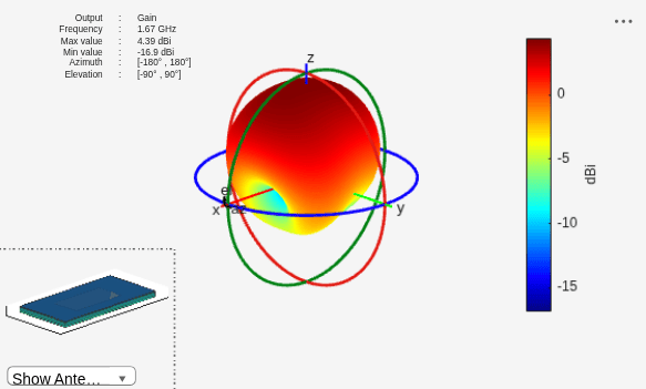
Plot the radiation pattern of the antenna.
figure pattern(p,1.67e9)
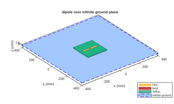
Design a dipole antenna backed by a dielectric substrate and an infinite reflector.
Create a dipole antenna of length, 0.15 m, and width, 0.015 m.
d = dipole(Length=0.15,Width=0.015,Tilt=90,TiltAxis=[0 1 0]);
Create a reflector using the dipole antenna as an exciter and the dielectric, teflon as the substrate.
t = dielectric("Teflon")t =
dielectric with properties:
Name: 'Teflon'
EpsilonR: 2.1000
LossTangent: 2.0000e-04
Thickness: 0.0060
FrequencyModel: 'Constant'
For more materials see catalog
rf = reflector(Exciter=d,Spacing=7.5e-3,Substrate=t);
Set the groundplane length of the reflector to inf. View the structure.
rf.GroundPlaneLength = inf; show(rf)
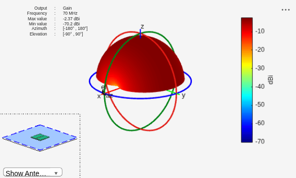
Calculate the radiation pattern of the antenna at 70 MHz.
pattern(rf,70e6)
Compare the gain values of a dipole antenna in free space and dipole antenna on a substrate.
Design a dipole antenna at a frequency of 1 GHz.
d = design(dipole,1e9); l_by_w = d.Length/d.Width; d.Tilt = 90; d.TiltAxis = [0 1 0];
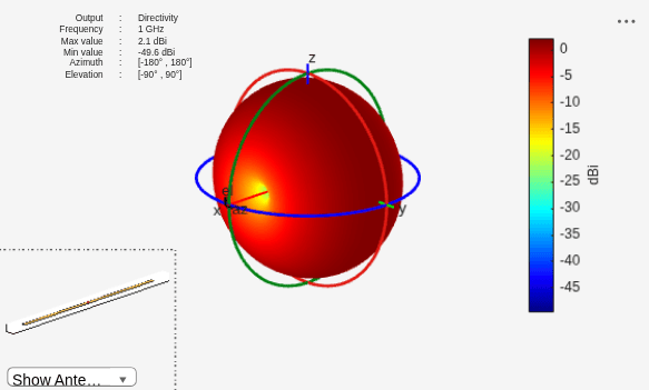
Plot the radiation pattern of the dipole in free space at 1 GHz.
figure pattern(d,1e9);
Use FR4 as the dielectric substrate.
t = dielectric("FR4")t =
dielectric with properties:
Name: 'FR4'
EpsilonR: 4.8000
LossTangent: 0.0260
Thickness: 0.0060
FrequencyModel: 'Constant'
For more materials see catalog
eps_r = t.EpsilonR;
lambda_0 = physconst("lightspeed")/1e9;
lambda_d = lambda_0/sqrt(eps_r);Adjust the length of the dipole based on the wavelength.
d.Length = lambda_d/2; d.Width = d.Length/l_by_w;
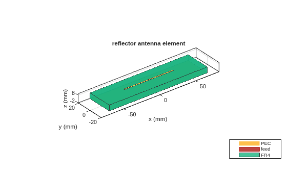
Design a reflector at 1 GHz with the dipole as the exciter and FR4 as the substrate.
rf = reflector(Exciter=d,Spacing=7.5e-3,Substrate=t); rf.GroundPlaneLength = lambda_d; rf.GroundPlaneWidth = lambda_d/4; figure show(rf)
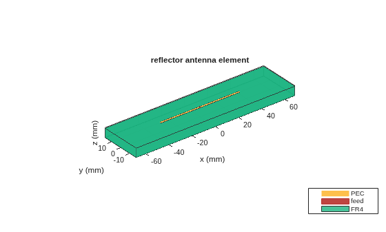
Remove the groundplane for plotting the gain of the dipole on the substrate.
rf.GroundPlaneLength = 0; show(rf)
Plot the radiation pattern of the dipole on the substrate at 1 GHz.
figure pattern(rf,1e9);
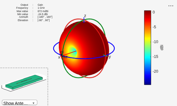
Compare the gain values.
Gain of the dipole in free space = 2.11 dBi
Gain of the dipole on substrate = 1.93 dBi
Version History
Introduced in R2016aThe TableDriven frequency dispersion model now returns the
EpsilonR and LossTangent values that you specify
directly at the corresponding Frequency points. The model applies a
rational fit only to interpolate between or extrapolate beyond those points. In previous
releases, the model applied a rational fit across all frequency points, so evaluating the
material at a specified frequency point could return values that differed from your
tabulated data.
The rational fit used for interpolation and extrapolation now requires an RF
Toolbox license. Without RF Toolbox, you can evaluate a
TableDriven material at its specified frequency points, but evaluating
it at other frequencies returns an error.
The dielectric object now lets you choose a dispersion model to
include the effect of frequency variation on the dielectric properties of the material. The
supported dispersion models are constant, Djordjevic-Sarkar, mean of Djordjevic-Sarkar, and
table driven. To specify a frequency for the dielectric, use the new
Frequency name-value argument. To specify a dispersion model, use the
new FrequencyModel name-value argument.
MATLAB Command
You clicked a link that corresponds to this MATLAB command:
Run the command by entering it in the MATLAB Command Window. Web browsers do not support MATLAB commands.
Select a Web Site
Choose a web site to get translated content where available and see local events and offers. Based on your location, we recommend that you select: .
You can also select a web site from the following list
How to Get Best Site Performance
Select the China site (in Chinese or English) for best site performance. Other MathWorks country sites are not optimized for visits from your location.
Americas
- América Latina (Español)
- Canada (English)
- United States (English)
Europe
- Belgium (English)
- Denmark (English)
- Deutschland (Deutsch)
- España (Español)
- Finland (English)
- France (Français)
- Ireland (English)
- Italia (Italiano)
- Luxembourg (English)
- Netherlands (English)
- Norway (English)
- Österreich (Deutsch)
- Portugal (English)
- Sweden (English)
- Switzerland
- United Kingdom (English)