Antenna Far-Field Visualization
This example shows how to visualize the far fields for antennas and antenna arrays. Radiation patterns can be plotted in Antenna Toolbox™ using the pattern function. The example explains different options available in the pattern function.
Create Yagi-Uda Antenna
Create the Yagi-Uda antenna in the default configuration.
ant = yagiUda;
figure
show(ant)
title("Yagi-Uda Antenna");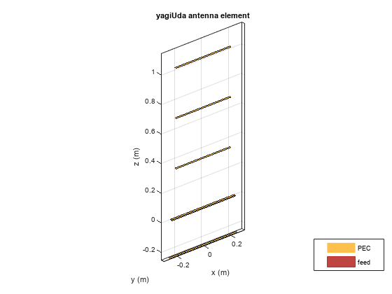
Plot Radiation Pattern
To plot the radiation pattern of the antenna, specify the frequency at which the data needs to be plotted. If no angles are provided, the azimuth spacing of 5 degrees between -180 to 180 degrees and the elevation spacing of 5 degrees from -90 to 90 degrees, respectively, are assumed. By default, the 3D antenna directivity is plotted expressed in decibels.
freq = 300e6;
pattern(ant,freq);
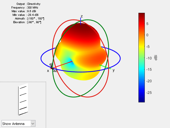
The list at top left corner of the figure window provides additional details such as minimum and maximum values of the quantity to be plotted as well as the range of angles where the data is plotted. In the lower left corner, there is the inset of the antenna. Rotating the radiation pattern rotates the antenna too. To remove the antenna image from the plot, clear the Show Antenna button.
Animate the Field in the E-plane
The analysis from the solver provides us with the steady state result. The field calculation provides the 3 components of the electric and magnetic field in phasor form in the cartesian coordinate system. Animate this field by using a propagator defined by the frequency, freq, to bring the result back to time-harmonic form and visualize on the E-plane and H-plane. In the case of the horn, E-plane is the XZ plane and H-plane is the XY plane. As noted in the far-field pattern plot shown in the previous section, the main lobe is along the positive x-axis. Use the helperAnimateEHFields function as shown below. Define the spatial extent, point density as well as the total number of time periods defined in terms of the frequency freq. Choose the Ez component with the plotting plane defined as XZ for the E-field. If the sampling time is not defined, the function automatically chooses a sampling time based on 10 times the center frequency. There is also an option available to save the animation output to a gif file with an appropriate name specified.
% Define Spatial Plane Extent
lambda = physconst("lightspeed")/freq;
SpatialInfo.XSpan = 5*lambda;
SpatialInfo.YSpan = 5*lambda;
SpatialInfo.ZSpan = 5*lambda;
SpatialInfo.NumPointsX = 400;
SpatialInfo.NumPointsY = 400;
SpatialInfo.NumPointsZ = 400;
% Define Time Extent
Tperiod = 1/freq;
T = 2*Tperiod;
TimeInfo.TotalTime = T;
TimeInfo.SamplingTime = [];
% Define E-Field Data details
DataInfo.Component = 'Ex';
DataInfo.PlotPlane = 'XZ';
DataInfo.DataLimits = [-2 6];
DataInfo.ScaleFactor = 1;
DataInfo.GifFileName = 'yagiEz.gif';
DataInfo.CloseFigure = true;
%% Animate
helperAnimateEHFields(ant,freq,SpatialInfo, TimeInfo, DataInfo)
Plot Individual Polarization Components
By default, the function pattern plots the overall directivity. To plot the directivity of the individual field components separately, use the Polarization flag. The options available are the directivity of the azimuthal electric field (H), the directivity of the elevation electric field (V), Right- handed circular polarization (RHCP) and Left Hand circular polarization (LHCP) components of the electric field. The plot below shows the directivity of the azimuthal component of the electric field.
pattern(ant,freq,Polarization="H");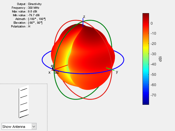
Plot 2D Patterns
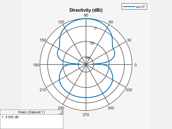
Individual slices of the directivity can be plotted using a polar or rectangular plot, to give a better understanding of how the field varies in different planes. The plot below shows the total directivity in the elevation plane (a 2D radiation pattern).
pattern(ant,freq,0,0:1:360);
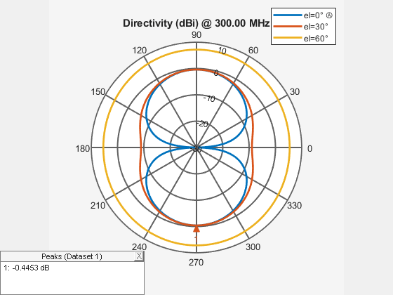
Use the patternAzimuth multiple patterns and overlay them on the single plot. The plot below shows three radiation patterns at azimuthal angles of 0, 30 and 60 degrees.
patternAzimuth(ant,freq,[0 30 60]);
To plot the patterns at fixed elevation angles, use the function patternElevation.
Directivity on a Rectangular Plot
The pattern function also allows us to visualize the patterns using a rectangular plot. This can be done by modifying the CoordinateSystem flag as shown below. By default, the flag is set to polar. Change it to rectangular to visualize the data in the rectangular coordinate system.
pattern(ant,freq,0:1:360,30,CoordinateSystem="rectangular");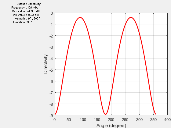
Plot Results at Multiple Frequencies
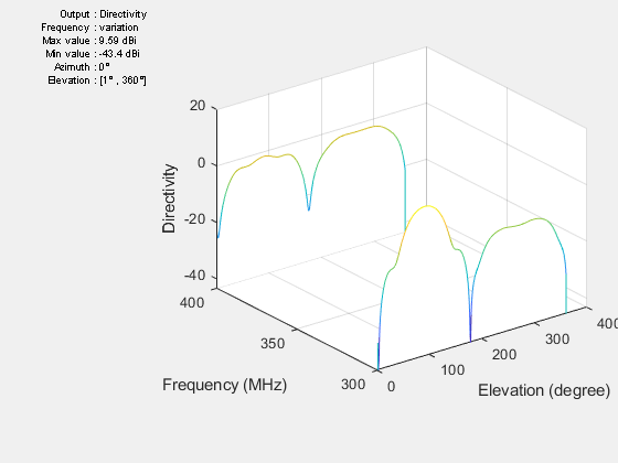
To plot patterns at multiple frequencies on the same graph, use the function pattern with the PlotStyle flag allowing a choice between Overlay or Waterfall style of plotting. The feature is important for the analysis of large-bandwidth antennas. The PlotStyle flag needs to be set to waterfall to display a waterfall plot. The default value of this flag is overlay.
pattern(ant,[300e6 400e6],0,1:1:360,PlotStyle="waterfall",...
    CoordinateSystem="rectangular");
U-V Plot
The third option for the CoordinateSystem flag is uv. This will plot the field data in the u-v coordinate system. The functionality is mostly useful for antenna arrays to visualize the array lobes.
pattern(ant,freq,CoordinateSystem="uv");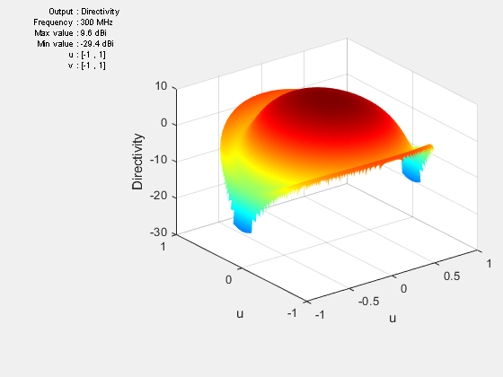
Plot Electric Field and Power
The pattern function also allows us to plot the linear field patterns. Different field quantities can be plotted by modifying the Type flag. By default it is set to directivity. It can be set to efield to plot the magnitude of the electric field. The plot below shows the normalized magnitude of the electric field.
pattern(ant,freq,Type="efield",Normalize=true);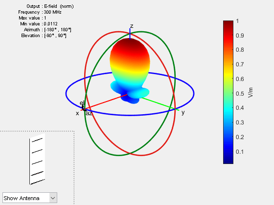
Beamwidth
The main beam is the region of the maximum radiation. In the present case, the main beam is along the z-axis. The half-power beamwidth (HPBW) is the angular separation in which the magnitude of the radiation pattern decreases by 50% (or -3dB) from the peak of the main beam. For example, we want to measure the width of the main beam in the elevation plane. The HPBW can be calculated as shown below
[bw, angles] = beamwidth(ant,freq,0,1:1:360)
bw =
52.0000
angles = 1×2

    64   116
The beamwidth is calculated at a single frequency and in a specified plane by choosing the respective values of azimuth or elevation angles. We observe that the width of the main beam is 52 degrees; the beam is located between 64 degrees and 116 degrees in the elevation plane.
References
[1] C. A. Balanis, 'Antenna Theory. Analysis and Design,' p. 514, Wiley, New York, 3rd Edition, 2005.
See Also
Antenna Near-Field Visualization | Plane Wave Excitation - Scattering Solution