Loading Using Lumped Elements
This example shows how to load an antenna using a lumped element. In other words, how to create a simple matching network by adding a lumped load at the feed. You can load an antenna to make it smaller, enable matching at the feedline, or to make the antenna larger to obtain higher performance. This example uses a cloverleaf antenna to demonstrate the impedance matching using the lumped element.
Create Cloverleaf Antenna
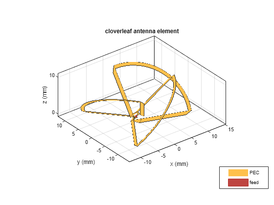
Create a cloverleaf antenna operating in the 5.5 to 6.05 GHz frequency range. A cloverleaf antenna is typically used on drones for communicating with the ground station or other drones in the vicinity.
ant = cloverleaf;
freq = linspace(5.5e9, 6.05e9, 51);
figure
show(ant)
Plot Impedance of Cloverleaf Antenna
Use the impedance function to plot the impedance of the antenna.
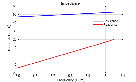
figure
impedance(ant,freq);
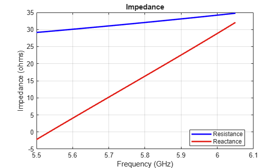
As seen from the impedance plot, the antenna resonates at 5.6GHz. The resistance and reactance value increases at higher frequencies. The impedance at 5.8 GHz is 32+ j12.
Plot Return Loss of Cloverleaf Antenna
Use the returnLoss function to plot return loss of the antenna.
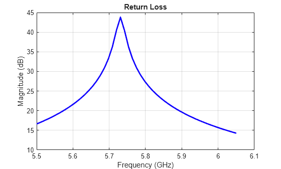
figure
returnLoss(ant,freq);
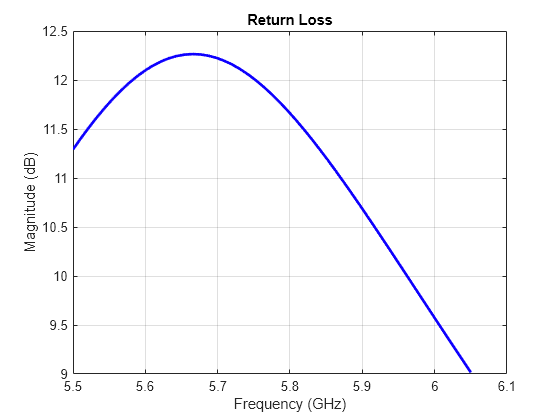
As evident from the return loss plot, the impedance matching at the lower frequencies (5.5 to 5.95 GHz) seems pretty good as return loss is greator than 10 dB. While at the higher frequencies (5.95 to 6.05 GHz), the return loss is less than 10dB and hence the matching is not good. This prevents the antenna from matching the specifications required for successful operation over the entire frequency range.
Define Lumped Element
The lumpedElement allows the user to specify a complex load. The load can be frequency independent (scalar) or dependent (vector). You can define the frequency variation as a vector using the Frequency property. This operating frequency range must match with the operating frequency range of the antenna loaded by this lumped element. You can also choose the location on the antenna surface where the load needs to be specified. The load is applied to the feed to achieve impedance matching.
le = lumpedElement
le =
  lumpedElement with properties:

    Impedance: []
    Frequency: []
     Location: 'feed'
Impedance Matching - Adding Load at Feed
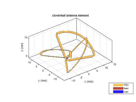
A better matching over the entire frequency range can be obtained by adding some impedance at the feed. As impedance variation is quite smooth a single impedance value might be enough to obtain a good match over the entire frequency range. Select the impedance at 5.8 GHz and match it exactly to 50 ohms using the lumpedElement. A blue dot is added at the feed indicating the location of the lumped load.
le.Impedance = complex(18,-12);
ant.Load = le;
figure
show(ant)
Calculate Impedance of Loaded Cloverleaf
Calculate the impedance of the lumped element loaded Cloverleaf antenna.
figure
impedance(ant,freq);
The impedance plot indicates that a constant 18 ohms is added to the resistance while a capacitive reactance of 12 ohms is added to the reactance over the entire frequency range. This also changes the resonant frequency of the antenna.
Calculate Return Loss of Loaded Cloverleaf
Calculate the return loss of the lumped element loaded Cloverleaf antenna.
figure
returnLoss(ant,freq);
However, changing the impedance over the entire frequency range does help with the impedance bandwidth. A value greater than 10 dB of return loss is seen over the entire frequency range of operation.
Add Load at Arbitrary Location on Antenna Surface
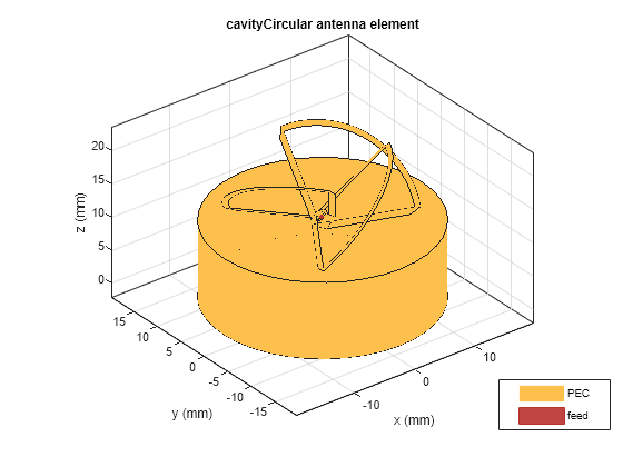
You can also load the antenna at an arbitrary location on the surface by specifying the x, y, and z coordinates of the location. Consider the same cloverleaf antenna but backed by a circular cavity as shown below.
ref = design(cavityCircular,5.5e9);
ref.Exciter = cloverleaf;
figure
show(ref)
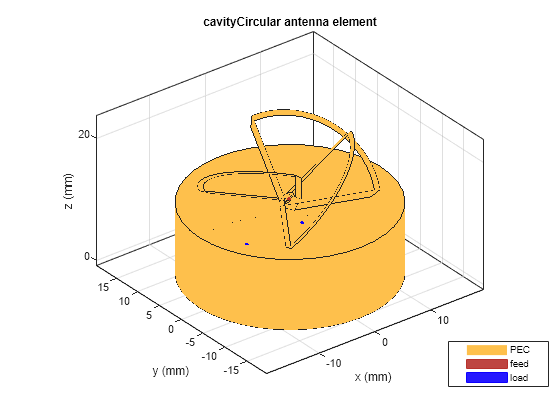
You can add some load to the cavity base to add more loss into the system. The blue dot added to the cavity base is the location of the lumped load.
refload = lumpedElement(Impedance=complex(20,20), Location=[0 10e-3 0]);
ref.Load = refload;
figure
show(ref)

Add Multiple Loads
Specify multiple lumped elements to add multiple loads to the antenna. You can specify these either at the feed or on the antenna surface. Multiple blue dots are observed on the antenna surface indicating the location of the load.
refload2 = lumpedElement(Impedance=complex(30,-10), Location=[10e-3, 10e-3, 0]);
ref.Load = [refload, refload2];
figure
show(ref)
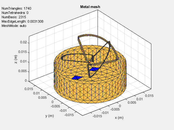
All the analysis performed on the above antenna takes into account the effect of the lumped load. This is done by adding the impedance value specified in the lumped load to the basis function in the interaction matrix of Method of Moments. The edge at which the load is added can be visualized by looking at the mesh. The common edge shared by the two blue triangles is the edge at which the impedance value gets added.
z = impedance(ref,5.5e9);
figure
mesh(ref);
See Also
Comparison of Antenna Array Transmit and Receive Manifold | Impedance Matching of Non-resonant (Small) Monopole