openl3
(Not recommended) OpenL3 neural network
openl3 is not recommended. Use the audioPretrainedNetwork function instead.
Description
net = openl3
This function requires both Audio Toolbox™ and Deep Learning Toolbox™.
net = openl3(Name,Value)net =
openl3('EmbeddingLength',6144) specifies the output embedding length as
6144.
Examples
Download and unzip the Audio Toolbox™ model for OpenL3.
Type openl3 at the Command Window. If the Audio Toolbox model for OpenL3 is not installed, the function provides a link to the location of the network weights. To download the model, click the link. Unzip the file to a location on the MATLAB® path.
Alternatively, execute these commands to download and unzip the OpenL3 model to your temporary directory.
downloadFolder = fullfile(tempdir,'OpenL3Download');
loc = websave(downloadFolder,'https://ssd.mathworks.com/supportfiles/audio/openl3.zip');
OpenL3Location = tempdir;
unzip(loc,OpenL3Location)
addpath(fullfile(OpenL3Location,'openl3'))
Check that the installation is successful by typing openl3 at the Command Window. If the network is installed, then the function returns a DAGNetwork (Deep Learning Toolbox) object.
openl3
ans =
  DAGNetwork with properties:

         Layers: [30×1 nnet.cnn.layer.Layer]
    Connections: [29×2 table]
     InputNames: {'in'}
    OutputNames: {'out'}
Load a pretrained OpenL3 convolutional neural network and examine the layers and classes.
Use openl3 to load the pretrained OpenL3 network. The output net is a DAGNetwork (Deep Learning Toolbox) object.
net = openl3
net =
  DAGNetwork with properties:

         Layers: [30×1 nnet.cnn.layer.Layer]
    Connections: [29×2 table]
     InputNames: {'in'}
    OutputNames: {'out'}
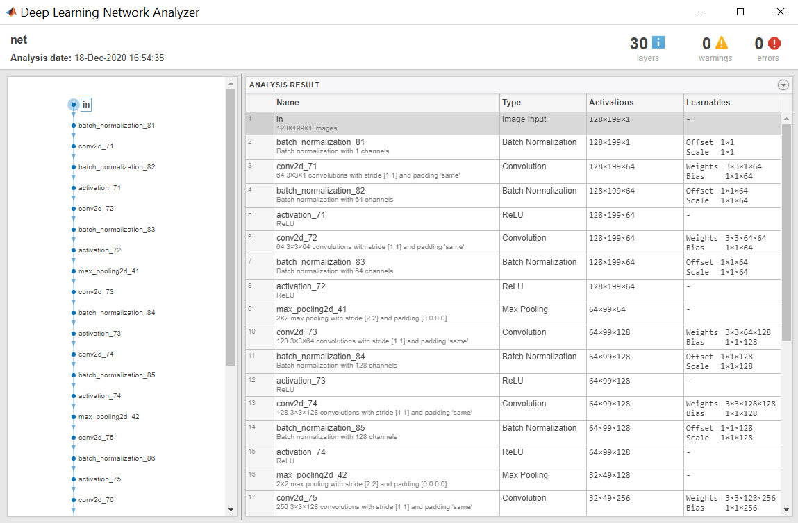
View the network architecture using the Layers property. The network has 30 layers. There are 16 layers with learnable weights, of which eight are batch normalization layers and eight are convolutional layers.
net.Layers
ans =
  30×1 Layer array with layers:

     1   'in'                       Image Input           128×199×1 images
     2   'batch_normalization_81'   Batch Normalization   Batch normalization with 1 channels
     3   'conv2d_71'                Convolution           64 3×3×1 convolutions with stride [1  1] and padding 'same'
     4   'batch_normalization_82'   Batch Normalization   Batch normalization with 64 channels
     5   'activation_71'            ReLU                  ReLU
     6   'conv2d_72'                Convolution           64 3×3×64 convolutions with stride [1  1] and padding 'same'
     7   'batch_normalization_83'   Batch Normalization   Batch normalization with 64 channels
     8   'activation_72'            ReLU                  ReLU
     9   'max_pooling2d_41'         Max Pooling           2×2 max pooling with stride [2  2] and padding [0  0  0  0]
    10   'conv2d_73'                Convolution           128 3×3×64 convolutions with stride [1  1] and padding 'same'
    11   'batch_normalization_84'   Batch Normalization   Batch normalization with 128 channels
    12   'activation_73'            ReLU                  ReLU
    13   'conv2d_74'                Convolution           128 3×3×128 convolutions with stride [1  1] and padding 'same'
    14   'batch_normalization_85'   Batch Normalization   Batch normalization with 128 channels
    15   'activation_74'            ReLU                  ReLU
    16   'max_pooling2d_42'         Max Pooling           2×2 max pooling with stride [2  2] and padding [0  0  0  0]
    17   'conv2d_75'                Convolution           256 3×3×128 convolutions with stride [1  1] and padding 'same'
    18   'batch_normalization_86'   Batch Normalization   Batch normalization with 256 channels
    19   'activation_75'            ReLU                  ReLU
    20   'conv2d_76'                Convolution           256 3×3×256 convolutions with stride [1  1] and padding 'same'
    21   'batch_normalization_87'   Batch Normalization   Batch normalization with 256 channels
    22   'activation_76'            ReLU                  ReLU
    23   'max_pooling2d_43'         Max Pooling           2×2 max pooling with stride [2  2] and padding [0  0  0  0]
    24   'conv2d_77'                Convolution           512 3×3×256 convolutions with stride [1  1] and padding 'same'
    25   'batch_normalization_88'   Batch Normalization   Batch normalization with 512 channels
    26   'activation_77'            ReLU                  ReLU
    27   'audio_embedding_layer'    Convolution           512 3×3×512 convolutions with stride [1  1] and padding 'same'
    28   'max_pooling2d_44'         Max Pooling           16×24 max pooling with stride [16  24] and padding 'same'
    29   'flatten'                  Keras Flatten         Flatten activations into 1-D assuming C-style (row-major) order
    30   'out'                      Regression Output     mean-squared-error
Use analyzeNetwork (Deep Learning Toolbox) to visually explore the network.
analyzeNetwork(net)
Use openl3Preprocess to extract embeddings from an audio signal.
Read in an audio signal.
[audioIn,fs] = audioread("Counting-16-44p1-mono-15secs.wav");To extract spectrograms from the audio, call the openl3Preprocess function with the audio and sample rate. Use 50% overlap and set the spectrum type to linear. The openl3Preprocess function returns an array of 30 spectrograms produced using an FFT length of 512.
features = openl3Preprocess(audioIn,fs,OverlapPercentage=50,SpectrumType="linear");
[posFFTbinsOvLap50,numHopsOvLap50,~,numSpectOvLap50] = size(features)
posFFTbinsOvLap50 = 257
numHopsOvLap50 =
197
numSpectOvLap50 =
30
Call openl3Preprocess again, this time using the default overlap of 90%. The openl3Preprocess function now returns an array of 146 spectrograms.
features = openl3Preprocess(audioIn,fs,SpectrumType="linear");
[posFFTbinsOvLap90,numHopsOvLap90,~,numSpectOvLap90] = size(features)
posFFTbinsOvLap90 = 257
numHopsOvLap90 =
197
numSpectOvLap90 =
146
Visualize one of the spectrograms at random.
randSpect = randi(numSpectOvLap90);
viewRandSpect = features(:,:,:,randSpect);
N = size(viewRandSpect,2);
binsToHz = (0:N-1)*fs/N;
nyquistBin = round(N/2);
semilogx(binsToHz(1:nyquistBin),mag2db(abs(viewRandSpect(1:nyquistBin))))
xlabel("Frequency (Hz)")
ylabel("Power (dB)");
title([num2str(randSpect),"th Spectrogram"])
axis tight
grid on

Create an OpenL3 network using the same SpectrumType.
net = audioPretrainedNetwork("openl3",SpectrumType="linear");
Extract and visualize the audio embeddings.
embeddings = predict(net,features);
surf(embeddings,EdgeColor="none")
view([90,-90])
axis([1 numSpectOvLap90 1 numSpectOvLap90])
xlabel("Embedding Length")
ylabel("Spectrum Number")
title("OpenL3 Feature Embeddings")
axis tight

Name-Value Arguments
Output Arguments
References
[1] Cramer, Jason, et al. "Look, Listen, and Learn More: Design Choices for Deep Audio Embeddings." In ICASSP 2019 IEEE International Conference on Acoustics, Speech and Signal Processing (ICASSP), IEEE, 2019, pp. 3852-56. DOI.org (Crossref), doi:/10.1109/ICASSP.2019.8682475.
Extended Capabilities
Version History
Introduced in R2021a