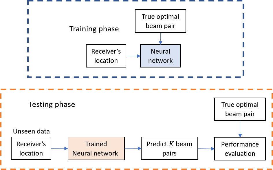
Neural Network for Beam Selection
This example shows how to use a neural network to reduce the overhead in the beam selection task. In the example, you use only the location of the receiver rather than knowledge of the communication channels. Instead of an exhaustive beam search over all the beam pairs, you can reduce beam sweeping overhead by searching among the selected beam pairs. Considering a system with a total of 70 beam pairs, simulation results show that the designed machine learning algorithm can achieve an accuracy of 90% by performing an exhaustive search over less than a quarter of the beam pairs. For the simulation, the example considers an urban macrocell (UMa) scenario, as defined in TR 38.901 and TR 38.843.
Introduction
To enable millimeter wave (mmWave) communications, you should use beam management techniques due to the high pathloss and blockage at high frequencies. Beam management is a set of Layer 1 (physical layer) and Layer 2 (medium access control) procedures that establish and retain an optimal beam pair (transmit beam and a corresponding receive beam) for good connectivity. For simulations of 5G New Radio (NR) beam management procedures, see the NR SSB Beam Sweeping and NR Downlink Transmit-End Beam Refinement Using CSI-RS examples.
This example considers beam selection procedures when a connection is established between the user equipment (UE) and access network node (gNB). In 5G NR, the beam selection procedure for initial access consists of beam sweeping, which requires exhaustive searches over all the beams on the transmitter and the receiver sides, and then selection of the beam pair offering the strongest reference signal received power (RSRP). Since mmWave communications require many antenna elements, implying many beams, an exhaustive search over all beams becomes computationally expensive and increases the initial access time.
To avoid repeatedly performing an exhaustive search and to reduce the communication overhead, you can apply machine learning to the beam selection problem. You can pose the beam selection problem as a classification task or a regression task. This example uses a regression approach where the network predicts RSRP values for all beam pairs, as discussed in TDoc R1-2306856. The network uses downsampled RSRP measurements to predict the full RSRP profile across all beam pairs. Specifically, given the reduced data set of downsampled RSRP measurements, a trained machine learning model recommends a set of good beam pairs. Instead of an exhaustive search over all the beam pairs, the simulation reduces beam sweeping overhead by searching only among the selected beam pairs.
This example uses a neural network to perform beam selection using downsampled RSRP measurements and a channel model compliant with the definition in TR 38.901. The example follows these three main steps:
1. Generate Training and Test Data
For each set of training and testing data, follow these steps:
Generate spatially consistent channels for UEs randomly dropped within the extents of a scenario compliant with the definition in TR 38.901. For each possible pair of synchronization signal block (SSB) beams between gNB and each UE, generate a waveform containing SSB and pass it through the channel.
Measure the value of the RSRP received by the UE for each beam pair.
Generate downsampled RSRP measurements by preprocessing the RSRP measurements via normalizing, reshaping, and downsampling.
Obtain the optimal beam pair for each UE by sorting all beam pairs for each UE based on their RSRP measurements.
2. Train the Neural Network
Using the generated training data, extract 10% of the data to be used as a validation set during the training of the neural network. The example uses the remaining 90% of the data for the training of the neural network.
Design and train a neural network that uses downsampled RSRP measurements as input and predicts the full RSRP vector across all beam pairs as output. The network learns to interpolate RSRP values from sparse measurements.

3. Test the Neural Network and Evaluate Its Performance
Using the generated test data, run the trained neural network to predict RSRP values across all beam pairs and UEs.
Select the top beam pairs with the highest predicted RSRP values.
Perform an exhaustive search over these beam pairs to find the one with the highest actual RSRP as the final prediction.
Evaluate the neural network performance by comparing the predicted best beam pair against the true known optimal beam pair. The example measures the effectiveness of the proposed method using two metrics: average RSRP and top- accuracy.

Generate Training and Test Data
In the prerecorded data, a channel is simulated where UEs are randomly distributed inside the first sector of a three-sector cell, as discussed in TR 38.901. The UE locations are used to generate the channel realizations and RSRP measurements, and are also used as input to the K-nearest neighbors (KNN) benchmark method. The example uses the baseline system-level simulation assumptions for AI/ML from TR 38.843 Table 6.3.1-1. The number of transmit and receive beams depends on the half-power beamwidth. While minimizing the number of beams, the example selects enough beams to cover the full area. By default, the example considers ten transmit beams and seven receive beams, according to the antenna specifications defined in TR 38.843 Table 6.3.1-1. After the TR 38.901 channel is set up, the example considers 20,000 different UE locations in the training set and 700 different UE locations in the test set. For each location, the example performs SSB-based beam sweeping for an exhaustive search over all 70 beam pairs and determines the true optimal beam pair by picking the beam pair with the highest RSRP.
To generate new training and test sets, you can adjust the useSavedData and SaveData check boxes.
useSavedData =true; saveData =
false; filenameParam = "nnBS_prm.mat"; filenameTrainData = "nnBS_TrainingData.mat"; filenameTestData = "nnBS_TestData.mat"; if useSavedData load(filenameParam); % Load beam selection system parameters load(filenameTrainData); % Load prerecorded training samples load(filenameTestData); % Load prerecorded test samples end
Define Data Generation Parameters
Configure the scenario by following the default values in TR 38.843 Table 6.3.1-1.
if ~useSavedData prm.NCellID =1; prm.FrequencyRange =
"FR2"; prm.Scenario =
"UMa"; prm.CenterFrequency =
30e9; % Hz prm.SSBlockPattern =
"Case D"; % Case A/B/C/D/E % Number of transmitted blocks. Set it to empty to let the example use % the minimum number that ensures a full coverage of the 120-degree % sector without overlapping of beams or gaps in the coverage prm.NumSSBlocks =
[]; prm.InterSiteDistance =
200; % meters prm.PowerBSs =
40; % dBm prm.UENoiseFigure =
10; % UE receiver noise figure in dB % Define the method to compute the RSRP: |SSSonly| uses SSS alone and % |SSSwDMRS| uses SSS and PBCH DM-RS. prm.RSRPMode =
"SSSwDMRS"; % Antenna array configuration c = physconst("LightSpeed"); % Propagation speed prm.Lambda = c/prm.CenterFrequency; % Wavelength prm.ElevationSweep = false; % Enable/disable elevation sweep % Define the transmit antenna array as a rectangular array with 4-by-8 % cross-polarized elements, as defined in TR 38.901. The example % considers the base station covering the first of a three-sector cell, % as defined in TR 38.901 Table 7.8-1, where the first sector is % centered at 30 degrees. Set the antenna sweep limits in azimuth to % cover the entire 120-degree sector, considering that the antenna % array points towards the center of the sector. prm.TransmitAntennaArray = phased.NRRectangularPanelArray( ... Size=[4,8,1,1], ... Spacing=[0.5,0.5,1,1]*prm.Lambda); % Transmit azimuth and elevation sweep limits in degrees prm.TxAZlim = [-60 60]; prm.TxELlim = [-90 0]; % Transmit antenna downtilt angle in degrees. The default value is % defined in TR 38.843 Table 6.3.1-2. prm.TxDowntilt = 110; % Define the receive antenna array as a rectangular array with 1-by-4 % omnidirectional cross-polarized elements, as defined in TR 38.901. % Set the antenna sweep limits in azimuth to cover half of the entire % 360-degree space, as the antenna array pattern is symmetrical and % antenna elements are omnidirectional. prm.ReceiveAntennaArray = phased.NRRectangularPanelArray( ... Size=[1,4,1,1], ... Spacing=[0.5,0.5,1,1]*prm.Lambda, ... ElementSet={phased.ShortDipoleAntennaElement, ... phased.ShortDipoleAntennaElement}); % Ensure the two elements are cross polarized with +45 and -45 deg % polarization angles prm.ReceiveAntennaArray.ElementSet{1}.AxisDirection = "Custom"; prm.ReceiveAntennaArray.ElementSet{1}.CustomAxisDirection = [0; 1; 1]; prm.ReceiveAntennaArray.ElementSet{2}.AxisDirection = "Custom"; prm.ReceiveAntennaArray.ElementSet{2}.CustomAxisDirection = [0; -1; 1]; % Receive azimuth and elevation sweep limits in degrees prm.RxAZlim = [-90 90]; prm.RxELlim = [0 90]; % Validate the current parameter set prm = validateParams(prm); if saveData % Save the parameters structure save(filenameParam,"prm"); end end
Generate Training Data
Set the number of UE locations for the training data. The hGenData38901Channel function randomly positions the specified number of UEs within the first sector boundaries of the cell.
if ~useSavedData
    prmTrain = prm;
    prmTrain.NumUELocations = 20e3;
    prmTrain.Seed = 42; % Set random number generator seed for repeatability

    % Generate the training data for each UE location
    disp("Generating training data ...")
    [optBeamPairIdxTrain,rsrpMatTrain,dataTrain] = hGenData38901Channel(prmTrain);
    disp("Finished generating training data.")

    if saveData
        % Save the training data
        save(filenameTrainData,"optBeamPairIdxTrain","rsrpMatTrain","dataTrain");
    end
end
Generate Testing Data
Set the number of UE locations for the testing data.
if ~useSavedData
    prmTest = prm;
    prmTest.NumUELocations = 700;
    prmTest.Seed = 24; % Set random number generator seed for repeatability

    % Generate the testing data for each UE location
    disp("Generating test data ...")
    [optBeamPairIdxTest,rsrpMatTest,dataTest] = hGenData38901Channel(prmTest);
    disp("Finished generating test data.")

    if saveData
        % Save the testing data
        save(filenameTestData,"optBeamPairIdxTest","rsrpMatTest","dataTest");
    end
end
Plot Transmitter and UE Locations
Plot training and testing data within the first sector of the cell, as defined in TR 38.901.
% Extract the UE and BS positions for training and testing data
positionsUE = {dataTrain.PosUE, dataTest.PosUE};
positionsBS = {dataTrain.PosBS, dataTest.PosBS};
plotLocations(positionsUE, positionsBS, prm.InterSiteDistance);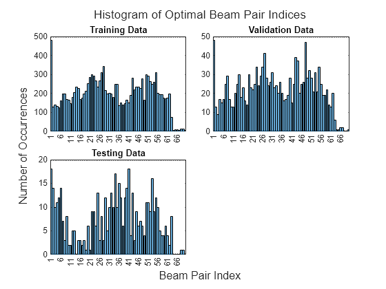
Process and Visualize Data
Preprocess the RSRP data to create inputs and outputs for the neural network, then visualize the spatial distribution and frequency of optimal beam pairs. The input of the network consists of downsampled RSRP measurements (every fifth beam pair), and the output of the network is the full RSRP vector across all beam pairs. This preprocessing enables the network to learn RSRP interpolation from sparse measurements.
Process Training Data
Extract optimal beam pair indices from RSRP data for visualization and benchmark analysis.
optBeamPairIdxScalarTrain = processData(prm,rsrpMatTrain);
Use 10% of training data as validation data.
totalTrainSamples = dataTrain.NumUELocations;
valDataLen = round(0.1*totalTrainSamples);
Randomly shuffle the training data such that the distribution of the extracted validation data is closer to the training data.
rng(111)
shuffledIdx = randperm(totalTrainSamples);
rsrpMatTrain = rsrpMatTrain(:,:,shuffledIdx);
locationMatTrain = dataTrain.PosUE(shuffledIdx, :);
Get the validation set.
rsrpMatVal = rsrpMatTrain(:,:,1:valDataLen);
Get the training set and location associated to it.
rsrpMatTrainMinusVal = rsrpMatTrain(:,:,valDataLen+1:end);
trainLocs = locationMatTrain(valDataLen+1:end,:);
Process Test Data
optBeamPairIdxScalarTest = processData(prm,rsrpMatTest);
Create Input and Output Data for Neural Network
Preprocess the RSRP data to create input and output for the neural network:
Normalize — To reduce the range of values, normalize all RSRP values by the global maximum absolute value from the training set.
Reshape — Convert 3-D arrays of
NumRxBeams-by-NumTxBeams-by-NumSamplesto 2-D arrays ofNumBeamPairs-by-NumSamples.Downsample — Create sparse RSRP measurements data for the training network input by selecting every fifth beam pair, in total 14 out of 70 beam pairs. The network output uses the full RSRP vector for all 70 beam pairs.
% Normalize
globalMax = max(abs(rsrpMatTrainMinusVal), [], "all");
globalMax = max(globalMax, eps);
normalize = @(x) x / globalMax;
rsrpMatTrainNorm = normalize(rsrpMatTrainMinusVal);
rsrpMatValNorm   = normalize(rsrpMatVal);
rsrpMatTestNorm  = normalize(rsrpMatTest);

% Reshape and downsample
numSampledBeams = 14;
numBeamPairs = prm.NumRxBeams*prm.NumTxBeams;
downsampleStep = round(numBeamPairs/numSampledBeams);
vec = @(x) reshape(x, numBeamPairs, []); % (RxTx)×N

% training
rsrpTrainVec      = vec(rsrpMatTrainNorm);
rsrpTrainInput    = rsrpTrainVec(1:downsampleStep:end, :);

% validation
rsrpValVec        = vec(rsrpMatValNorm);
rsrpValInput      = rsrpValVec(1:downsampleStep:end, :);

% test
rsrpTestVec       = vec(rsrpMatTestNorm);
rsrpTestInput     = rsrpTestVec(1:downsampleStep:end, :);
Create test input for KNN benchmark from the UE locations. Note that the neural network uses RSRP measurements, not locations.
testLocs = dataTest.PosUE;
Plot Histogram for Optimal Beam Pairs
Plot a histogram that shows how many times each beam pair is optimal. If some beam pairs are never optimal, try increasing the training and testing data set by increasing the number of UE locations.
data = {optBeamPairIdxScalarTrain(valDataLen+1:end), ...
    optBeamPairIdxScalarTrain(1:valDataLen), ...
    optBeamPairIdxScalarTest};
plotBeamPairsHist(data);
Design and Train Neural Network
This example uses the neural network described in TDoc R1-2306856. The neural network uses a regression approach with four hidden layers (64-128-256-128 neurons) and ReLU activations, followed by a tanh output activation. It takes 14 downsampled RSRP measurements as input and predicts a full 70-element RSRP vector as output, effectively learning to interpolate channel quality across all beam pairs from sparse measurements. The network is trained using MSE loss to minimize prediction error between predicted and actual RSRP values. During inference, the top- beam pairs with the highest predicted RSRP values are selected for beam sweeping.
To enable training, select the trainNow check box.
Modify the network to experiment with different designs. If you modify one of the provided data sets, you must retrain the network with the modified data sets. To use the trained network in subsequent runs, select the saveNet check box.
trainNow =false; saveNet =
false; filenameNet = "nnBS_trainedNet.mat";
If the trainNow check box is not selected, load the pretrained network.
if ~trainNow
    load(filenameNet);
end
If the trainNow check box is selected, design and train the neural network.
if trainNow
    % Neural network design
    layers = dlnetwork([ ...
        featureInputLayer(numSampledBeams,Name="input")

        fullyConnectedLayer(64,Name="linear1")
        reluLayer(Name="relu1")

        fullyConnectedLayer(128,Name="linear2")
        reluLayer(Name="relu2")

        fullyConnectedLayer(256,Name="linear3")
        reluLayer(Name="relu3")

        fullyConnectedLayer(128,Name="linear4")
        reluLayer(Name="relu4")

        fullyConnectedLayer(numBeamPairs,Name="linear5")
        tanhLayer(Name="tanh1")]); % Regression output

    % Set the maxEpochs to 500 and InitialLearnRate to 1e-4 to avoid
    % overfitting the network to the training data
    maxEpochs = 500;
    miniBatchSize = 200;

    % Set the training execution environment to "gpu" if a GPU is available,
    % to "parallel-auto" if a GPU is not available but the Parallel Computing
    % Toolbox(TM) is available, or to "cpu" otherwise
    if canUseGPU()
        execEnv = "gpu";
    elseif canUseParallelPool()
        execEnv = "parallel-auto";
    else
        execEnv = "cpu";
    end

    % Define the training options
    options = trainingOptions("adam", ...
        MaxEpochs=maxEpochs, ...
        MiniBatchSize=miniBatchSize, ...
        InitialLearnRate=1e-4, ...
        LearnRateSchedule="piecewise", ...
        LearnRateDropPeriod=10, ...
        LearnRateDropFactor=0.8, ...
        ValidationData={rsrpValInput,rsrpValVec}, ...
        ValidationFrequency=500, ...
        OutputNetwork="best-validation-loss", ...
        InputDataFormats="CB", ...
        TargetDataFormats="CB", ...
        Shuffle="every-epoch", ...
        Plots="training-progress", ...
        Verbose=false, ...
        ExecutionEnvironment=execEnv);

    % Train the network and show training information when training is
    % finished
    [net, netinfo] = trainnet(rsrpTrainInput, rsrpTrainVec, ...
        layers, @(x,t)mse(x,t), options);
    if saveNet
        % Save the network
        save(filenameNet,"net","netinfo");
    end
    disp(netinfo);
end
Compare Different Approaches: Top- Accuracy
This section evaluates the trained network on new test data using the top- accuracy metric. The top- accuracy metric is widely used in the neural network-based beam selection task.
Given downsampled RSRP measurements for a test sample, the neural network predicts RSRP values for all beam pairs and selects the top beam pairs with the highest predicted RSRP. Then it performs an exhaustive sequential search on these beam pairs and selects the one with the highest actual measured RSRP as the final prediction. If the true optimal beam pair is the final selected beam pair, then a successful prediction occurs. Equivalently, a success occurs when the true optimal beam pair is one of the recommended beam pairs by the neural network.
To use as benchmarks, the example implements three other methods to find the optimal beam pair indices. Each method produces the recommended beam pairs.
KNN — For a test sample, this method first collects closest training samples based on UE location coordinates. The method then recommends all the beam pairs associated with these training samples. Since each training sample has a corresponding optimal beam pair, the number of recommended beam pairs is at most (some beam pairs might be the same).
Statistical Info [7] — This method first ranks all the beam pairs according to their relative frequency in the testing set, and then selects the first beam pairs.
Random [7] — For a test sample, this method randomly chooses beam pairs.
The plot shows that for , the accuracy is already more than 90%, which highlights the effectiveness of using the trained neural network for the beam selection task. When , the Statistical Info scheme becomes an exhaustive search over all the 70 beam pairs. Hence, the Statistical Info scheme achieves an accuracy of 100%. However, when , KNN considers 70 closest training samples, and the number of distinct beam pairs from these samples is often less than 70. Therefore, KNN does not achieve an accuracy of 100%.
rng(111)    % for repeatability of the "Random" policy
statisticCount = accumarray(optBeamPairIdxScalarTrain, 1, [numBeamPairs, 1]);
predTestOutput = predict(net,rsrpTestInput, ...
    InputDataFormats="CB", OutputDataFormats="CB");

K = numBeamPairs;
accNeural = zeros(1,K);
accKNN = zeros(1,K);
accStatistic = zeros(1,K);
accRandom = zeros(1,K);
testDataLen = size(rsrpMatTestNorm,3);
for k = 1:K
    predCorrectNeural = zeros(testDataLen,1);
    predCorrectKNN = zeros(testDataLen,1);
    predCorrectStats = zeros(testDataLen,1);
    predCorrectRandom = zeros(testDataLen,1);
    knnIdx = knnsearch(trainLocs,testLocs,K=k);

    for n = 1:testDataLen
        % True optimal beam pair
        [~, trueOptBeamIdx] = max(rsrpMatTest(:,:,n), [], "all", "linear");

        % Neural Network
        [~, topKPredOptBeamIdx] = maxk(predTestOutput(:, n),k);
        if any(topKPredOptBeamIdx == trueOptBeamIdx)
            % if true, then the true correct index belongs to one of the K predicted indices
            predCorrectNeural(n,1) = true;
        end

        % KNN
        neighborsIdxInTrainData = knnIdx(n,:);
        topKPredOptBeamIdx= optBeamPairIdxScalarTrain(neighborsIdxInTrainData);
        if any(topKPredOptBeamIdx == trueOptBeamIdx)
            % if true, then the true correct index belongs to one of the K predicted indices
            predCorrectKNN(n,1) = true;
        end

        % Statistical Info
        [~, topKPredOptBeamIdx] = maxk(statisticCount,k);
        if any(topKPredOptBeamIdx == trueOptBeamIdx)
            % if true, then the true correct index belongs to one of the K predicted indices
            predCorrectStats(n,1) = true;
        end

        % Random
        topKPredOptBeamIdx = randperm(numBeamPairs,k);
        if any(topKPredOptBeamIdx == trueOptBeamIdx)
            % if true, then the true correct index belongs to one of the K predicted indices
            predCorrectRandom(n,1) = true;
        end

    end

    accuracy = @(x) nnz(x)/testDataLen*100;
    accNeural(k)    = accuracy(predCorrectNeural);
    accKNN(k)       = accuracy(predCorrectKNN);
    accStatistic(k) = accuracy(predCorrectStats);
    accRandom(k)    = accuracy(predCorrectRandom);

end
Plot the results.
results = {accNeural, accKNN, accStatistic, accRandom};
plotResults(results,K);
ylabel("Top-$K$ Accuracy (\%)",Interpreter="latex");
legend("Neural Network","KNN","Statistical Info","Random",Location="best");
Compare Different Approaches: Average RSRP
Using new test data, compute the average RSRP achieved by the neural network and the three benchmarks.
rng(111)    % for repeatability of the "Random" policy
K = numBeamPairs;
rsrpOptimal = zeros(1,K);
rsrpNeural = zeros(1,K);
rsrpKNN = zeros(1,K);
rsrpStatistic = zeros(1,K);
rsrpRandom = zeros(1,K);
for k = 1:K
    rsrpSumOpt = 0;
    rsrpSumNeural = 0;
    rsrpSumKNN = 0;
    rsrpSumStatistic = 0;
    rsrpSumRandom = 0;

    knnIdx = knnsearch(trainLocs,testLocs,K=k);

    for n = 1:testDataLen
        % Exhaustive Search
        [~, trueOptBeamIdx] = max(rsrpTestVec(:, n));
        rsrp = rsrpMatTest(:,:,n);
        rsrpSumOpt = rsrpSumOpt + rsrp(trueOptBeamIdx);

        % Neural Network
        [~, topKPredOptCatIdx] = maxk(predTestOutput(:, n),k);
        rsrpSumNeural = rsrpSumNeural + max(rsrp(topKPredOptCatIdx));

        % KNN
        neighborsIdxInTrainData = knnIdx(n,:);
        topKPredOptBeamIdxKNN = optBeamPairIdxScalarTrain(neighborsIdxInTrainData);
        rsrpSumKNN = rsrpSumKNN + max(rsrp(topKPredOptBeamIdxKNN));

        % Statistical Info
        [~, topKPredOptCatIdxStat] = maxk(statisticCount,k);
        rsrpSumStatistic = rsrpSumStatistic + max(rsrp(topKPredOptCatIdxStat));

        % Random
        topKPredOptBeamIdxRand = randperm(numBeamPairs,k);
        rsrpSumRandom = rsrpSumRandom + max(rsrp(topKPredOptBeamIdxRand));
    end
    rsrpOptimal(k)   = rsrpSumOpt/testDataLen;
    rsrpNeural(k)    = rsrpSumNeural/testDataLen;
    rsrpKNN(k)       = rsrpSumKNN/testDataLen;
    rsrpStatistic(k) = rsrpSumStatistic/testDataLen;
    rsrpRandom(k)    = rsrpSumRandom/testDataLen;
end
Plot the results. The plot shows that using the trained neural network results in an average RSRP closer to the optimal exhaustive search than using the other methods.
results = {rsrpNeural, rsrpKNN, rsrpStatistic, rsrpRandom, rsrpOptimal};
plotResults(results,K);
ylabel("Average RSRP");
legend("Neural Network","KNN","Statistical Info","Random","Exhaustive Search",Location="best");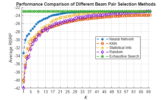
Compare the RSRP values for the optimal, neural network, and KNN approaches for the last four values ( to ).
table(rsrpOptimal(end-3:end)', rsrpNeural(end-3:end)', rsrpKNN(end-3:end)', VariableNames=["Optimal","Neural Network","KNN"])
ans=4×3 table
    Optimal    Neural Network      KNN
    _______    ______________    _______

    -24.059       -24.059        -24.691
    -24.059       -24.059         -24.68
    -24.059       -24.059        -24.659
    -24.059       -24.059        -24.649
The performance gap between KNN and the optimal methods indicates that the KNN might not perform well even when a larger set of beam pairs is considered, say, 256.
Further Exploration
This example describes the application of a regression-based neural network to the beam selection task for a 5G NR system. You can design and train a neural network that predicts RSRP values across all beam pairs from sparse measurements, enabling selection of the top beam pairs with the highest predicted RSRP. Beam sweeping overhead can be reduced by an exhaustive search only on those selected beam pairs.
The example enables you to specify the number of UE locations in the TR 38.901 channel. To see the impact of the channel on the beam selection, experiment with different scenarios, antenna elevation sweeping, and number of transmit and receive beams. The example also provides presaved data sets that you can use to experiment with different network structures and training hyperparameters.
From simulation results, for the prerecorded TR 38.901 channel for 70 beam pairs, the proposed algorithm achieves a top- accuracy of 90% when . This result demonstrates that by using the neural network, you can perform the exhaustive search over less than a quarter of all the beam pairs, which reduces the beam sweeping overhead by almost 80%. Experiment with varying other system parameters to see the efficacy of the network by regenerating data, then retraining and retesting the network.
References
3GPP TR 38.802, "Study on New Radio access technology physical layer aspects," 3rd Generation Partnership Project; Technical Specification Group Radio Access Network.
3GPP TR 38.843, "Study on Artificial Intelligence (AI)/Machine Learning (ML) for NR air interface," 3rd Generation Partnership Project; Technical Specification Group Radio Access Network.
3GPP TR 38.901, "Study on channel model for frequencies from 0.5 to 100 GHz," 3rd Generation Partnership Project; Technical Specification Group Radio Access Network.
TDoc R1-2306856, Intel Corporation, "Evaluation for AI/ML Beam Management," 3GPP TSG RAN WG1 #114, Toulouse, France, Aug 21st – 25th, 2023.
Klautau, A., González-Prelcic, N., and Heath, R. W., "LIDAR data for deep learning-based mmWave beam-selection," IEEE Wireless Communications Letters, vol. 8, no. 3, pp. 909–912, Jun. 2019.
Klautau, A., Batista, P., González-Prelcic, N., Wang, Y., and Heath, R. W., "5G MIMO Data for Machine Learning: Application to Beam-Selection Using Deep Learning," 2018 Information Theory and Applications Workshop (ITA), 2018, pp. 1–9, doi: 10.1109/ITA.2018.8503086.
Matteo, Z., PS-012-ML5G-PHY-Beam-Selection_BEAMSOUP (Team achieving the highest test score in the ITU Artificial Intelligence/Machine Learning in 5G Challenge in 2020).
Sim, M. S., Lim, Y., Park, S. H., Dai, L., and Chae, C., "Deep Learning-Based mmWave Beam Selection for 5G NR/6G With Sub-6 GHz Channel Information: Algorithms and Prototype Validation," IEEE Access, vol. 8, pp. 51634–51646, 2020.
Local Functions
function prm = validateParams(prm) %#ok<*DEFNU>
    % Validate user specified parameters and return updated parameters
    %
    % Only cross-dependent checks are made for parameter consistency.

    if strcmpi(prm.FrequencyRange,"FR1")
        if prm.CenterFrequency > 7.125e9 || prm.CenterFrequency < 410e6
            error("Specified center frequency is outside the FR1 " + ...
                "frequency range (410 MHz - 7.125 GHz).");
        end
        if any(strcmpi(prm.SSBlockPattern,["Case D","Case E"]))
            error("Invalid SSBlockPattern for selected FR1 frequency " + ...
                "range. SSBlockPattern must be one of 'Case A' or " + ...
                "'Case B' or 'Case C' for FR1.");
        end
        if (prm.CenterFrequency <= 3e9) && (length(prm.SSBTransmitted)~=4)
            error("SSBTransmitted must be a vector of length 4 for " + ...
                "center frequency less than or equal to 3GHz.");
        end
        if (prm.CenterFrequency > 3e9) && (length(prm.SSBTransmitted)~=8)
            error("SSBTransmitted must be a vector of length 8 for " + ...
                "center frequency greater than 3GHz and less than " + ...
                "or equal to 7.125GHz.");
        end
    else % "FR2"
        if prm.CenterFrequency > 52.6e9 || prm.CenterFrequency < 24.25e9
            error("Specified center frequency is outside the FR2 " + ...
                "frequency range (24.25 GHz - 52.6 GHz).");
        end
        if ~any(strcmpi(prm.SSBlockPattern,["Case D","Case E"]))
            error("Invalid SSBlockPattern for selected FR2 frequency " + ...
                "range. SSBlockPattern must be either 'Case D' or " + ...
                "'Case E' for FR2.");
        end
    end

    % Verify that there are multiple TX and Rx antennas
    prm.NumTx = getNumElements(prm.TransmitAntennaArray);
    prm.NumRx = getNumElements(prm.ReceiveAntennaArray);
    if prm.NumTx==1 || prm.NumRx==1
        error("Number of transmit or receive antenna elements must be greater than 1.");
    end

    % Number of beams at transmit end
    % Assume a number of beams so that the beams span the entire 120-degree
    % sector, with a maximum of 64 beams, as mentioned in TR 38.843 Table
    % 6.3.1-1
    % Assume the number of transmitted blocks is the same as the number of
    % beams at transmit end
    if prm.FrequencyRange=="FR1"
        maxNumSSBBlocks = 8;
    else % FR2
        maxNumSSBBlocks = 64;
    end
    if isempty(prm.NumSSBlocks)
        % The number of blocks/beams is automatically generated as the
        % minimum need to span the 120-degree sector
        azTxBW = beamwidth(prm.TransmitAntennaArray,prm.CenterFrequency,Cut="Azimuth");
        numAZTxBeams = round(diff(prm.TxAZlim)/azTxBW);

        if prm.ElevationSweep
            % If elevation sweep is enabled, consider elevation as well in
            % the computation of the number of blocks/beams needed.
            elTxBW = beamwidth(prm.TransmitAntennaArray,prm.CenterFrequency,Cut="Elevation");
            numELTxBeams = round(diff(prm.TxELlim)/elTxBW);
        else
            numELTxBeams = 1;
        end

        prm.NumTxBeams = min(numAZTxBeams*numELTxBeams, maxNumSSBBlocks);
        prm.NumSSBlocks = prm.NumTxBeams;
    else
        % The number of blocks/beams is defined by the user
        if prm.NumSSBlocks>maxNumSSBBlocks
            error("Invalid number of SSB blocks. For " + prm.FrequencyRange + ...
                ", there can be only up to " + maxNumSSBBlocks + " blocks.");
        end
        prm.NumTxBeams = prm.NumSSBlocks;
    end
    prm.SSBTransmitted = [ones(1,prm.NumTxBeams) zeros(1,maxNumSSBBlocks-prm.NumTxBeams)];

    % Number of beams at receive end
    % Assume a number of beams so that the beams cover the full azimuth
    % sweep, with a maximum of 8 beams, as mentioned in TR 38.843 Table
    % 6.3.1-1.
    azRxBW = beamwidth(prm.ReceiveAntennaArray,prm.CenterFrequency,Cut="Azimuth");
    numAZRxBeams = round(diff(prm.RxAZlim)/azRxBW);
    if prm.ElevationSweep
        % If elevation sweep is enabled, consider elevation as well in
        % the computation of the number of blocks/beams needed.
        elRxBW = beamwidth(prm.ReceiveAntennaArray,prm.CenterFrequency,Cut="Elevation");
        numELRxBeams = round(diff(prm.RxELlim)/elRxBW);
    else
        numELRxBeams = 1;
    end
    prm.NumRxBeams = min(numAZRxBeams*numELRxBeams, 8);

    % Select SCS based on SSBlockPattern
    switch lower(prm.SSBlockPattern)
        case "case a"
            scs = 15;
            cbw = 10;
            scsCommon = 15;
        case {"case b", "case c"}
            scs = 30;
            cbw = 25;
            scsCommon = 30;
        case "case d"
            scs = 120;
            cbw = 100;
            scsCommon = 120;
        case "case e"
            scs = 240;
            cbw = 200;
            scsCommon = 120;
    end
    prm.SCS = scs;
    prm.ChannelBandwidth = cbw;
    prm.SubcarrierSpacingCommon = scsCommon;

    % Set up SSBurst configuration
    txBurst = nrWavegenSSBurstConfig;
    txBurst.BlockPattern = prm.SSBlockPattern;
    txBurst.TransmittedBlocks = prm.SSBTransmitted;
    txBurst.Period = 20;
    txBurst.SubcarrierSpacingCommon = prm.SubcarrierSpacingCommon;
    prm.TxBurst = txBurst;
end

function optBeamPairIdxScalar = processData(prm,rsrpMat)
    % Extract optimal beam pair indices from RSRP measurements. Returns the
    % scalar representation of the optimal beam pair for each UE location,
    % as determined by the highest RSRP value.

    % Reshape rsrpMat from (NumRxBeams, NumTxBeams, NumLocations)
    % to (NumBeamPairs, NumLocations)
    numBeamPairs = prm.NumRxBeams*prm.NumTxBeams;
    rsrpReshaped = reshape(rsrpMat, numBeamPairs, []);

    % Find the beam pair index with max RSRP for each location
    [~, optBeamPairIdxScalar] = max(rsrpReshaped, [], 1);
    optBeamPairIdxScalar = optBeamPairIdxScalar(:);  % Convert to column vector
end

function plotLocations(positionsUE,positionsBS,ISD)
    % Plot UE and BS 2-D locations within the cell boundaries

    % Compute the cell boundaries
    [sitex,sitey] = h38901Channel.sitePolygon(ISD);

    % Plot training and testing data
    t = tiledlayout(TileSpacing="compact", GridSize=[1,2]);
    titles = ["Training Data", "Testing Data"];
    for idx = 1:numel(titles)
        nexttile
        plot(sitex,sitey,"--");
        box on;
        hold on;
        plot(positionsUE{idx}(:,1), positionsUE{idx}(:,2), "b.");
        plot(positionsBS{idx}(:,1), positionsBS{idx}(:,2), "^", MarkerEdgeColor="r", MarkerFaceColor="r");
        xlabel("x (m)");
        ylabel("y (m)");
        xlim([min(sitex)-10 max(sitex)+10]);
        ylim([min(sitey)-10 max(sitey)+10]);
        axis("square");
        title(titles(idx));
    end
    title(t, "Transmitter and UEs 2-D Positions");
    l = legend("Cell boundaries","UEs","Transmitter");
    l.Layout.Tile = "south";
end

function plotBeamPairsHist(data)
    % Plot the optimal beam pair histogram

    % Create tiled layout with 2x2 grid
    t = tiledlayout(2, 2, 'TileSpacing', 'compact');

    % Configuration
    titles = ["Training Data", "Validation Data", "Testing Data"];
    tileSpecs = {[1 2], 3, 4};  % Tile specifications for each plot

    % Create plots
    for idx = 1:numel(titles)
        nexttile(tileSpecs{idx});
        histogram(data{idx});
        title(titles(idx));
    end
    title(t, "Histogram of Optimal Beam Pair Indices");
    xlabel(t, "Beam Pair Index");
    ylabel(t, "Number of Occurrences");
end

function plotResults(results,K)
    % Plot the results from the comparison of different beam pair selection
    % methods

    figure
    lineWidth = 1.5;
    markerStyle = ["*","o","s","d","h"];
    hold on
    for idx = 1:numel(results)
        plot(1:K,results{idx},LineStyle="--",LineWidth=lineWidth,Marker=markerStyle(idx));
    end
    hold off
    grid on
    xticks([1 3 5 10 15:5:K]); % Explicitly highlight the top-K values in the plot
    xlabel("$K$",Interpreter="latex");
    title("Performance Comparison of Different Beam Pair Selection Methods");
end
See Also
Functions
featureInputLayer(Deep Learning Toolbox) |fullyConnectedLayer(Deep Learning Toolbox) |reluLayer(Deep Learning Toolbox) |trainNetwork(Deep Learning Toolbox) |trainingOptions(Deep Learning Toolbox)
Objects
phased.ULA(Phased Array System Toolbox) |phased.URA(Phased Array System Toolbox) |phased.IsotropicAntennaElement(Phased Array System Toolbox)
Topics
- Deep Learning in MATLAB (Deep Learning Toolbox)
- NR SSB Beam Sweeping
- NR Downlink Transmit-End Beam Refinement Using CSI-RS