Normalized Mean Squared Error as a Distance Measure
This example shows how to use the normalized mean squared error (NMSE) as a loss function for training a neural network in a wireless communications application.
Introduction
In wireless communications, accurately predicting signal behavior and performance is crucial for optimizing system design and operation. Neural networks have emerged as powerful tools for modeling and predicting complex relationships in communication systems. One critical aspect of training neural networks is the choice of the loss function, which guides the optimization process to minimize prediction errors.
The NMSE is an Euclidean distance measure similar to the mean squared error (MSE) . NMSE is particularly useful in scenarios where the scale of the data varies, as it normalizes the MSE by the variance of the target data, providing a scale-independent measure of prediction accuracy.
This example uses the helperNNDPDTrainingData function to generate data for the communications link. The signals x and y are the input and output of a power amplifier (PA). Ideally, the signals x and y should be the same, when the amplifier gain is removed. For more information see the Neural Network for Digital Predistortion Design-Offline Training example.
dpdData = helperNNDPDTrainingData;
x = dpdData.txWaveTrain;
y = dpdData.paOutputTrain;
Examine the signals.
plotSignals(x,y);
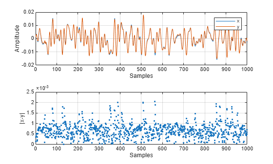
fprintf("The maximum amplitude of the signals is %f",max(max(abs(x)),max(abs(y))))The maximum amplitude of the signals is 0.020772
fprintf("The maximum absolute error between the two signals is %e",max(abs(x-y)))The maximum absolute error between the two signals is 2.052652e-03
fprintf("The average power of signal x is %e",mean(abs(x).^2))The average power of signal x is 7.787301e-05
Similarity Measures Based on Euclidean Distance
Measure the similarity of two signals using mean squared error (MSE) and normalized mean squared error (NMSE).
MSE Between Two Signals
MSE is defined as
.
mse = mean(abs(x-y).^2)
mse = single

5.6925e-07
In dB scale, MSE is
mse_dB = 10*log10(mse)
mse_dB = single

-62.4470
Since the amplitude and average power of signal x is small, MSE is also a very small number.
NMSE Between Two Signals
During training, small valued signals may not be taken into account as much as the larger valued signals. The NMSE loss function solves this problem by scaling the loss function with the signal power. The helperNMSE function implements the following equation and outputs NMSE in dB.
nmse = helperNMSE(x,y)
nmse = single

-21.3609
Train with NMSE and MSE
Train a neural network DPD using MSE and NMSE as loss function. Use the built in mse loss function and the custom helperNMSE function. First get the training options and the network using the helperNNDPDTrainingOptions function.
[net,options] = helperNNDPDTrainingOptions;
Set the random number generator to a known value to start training for both cases at the same initial conditions.
rng(123)
netDPDMSE = trainnet(dpdData.trainingInput,dpdData.trainingOutput, ...
  net,"mse",options);
    Iteration    Epoch    TimeElapsed    LearnRate    TrainingLoss
    _________    _____    ___________    _________    ____________
            1        1       00:00:00        0.001          3.4093
          256        2       00:00:02        0.001        0.015105
          512        4       00:00:02        0.001       0.0069223
          768        6       00:00:03      0.00095       0.0043773
         1024        8       00:00:04      0.00095       0.0025694
         1280       10       00:00:05      0.00095       0.0014847
         1536       12       00:00:06    0.0009025       0.0012758
         1792       14       00:00:07    0.0009025       0.0010268
         2048       16       00:00:07   0.00085737      0.00078196
         2304       18       00:00:08   0.00085737       0.0007438
         2560       20       00:00:09   0.00085737      0.00069718
Training stopped: Max epochs completed
rng(123)
netDPDNMSE = trainnet(dpdData.trainingInput,dpdData.trainingOutput, ...
  net,@(Y,T)helperNMSE(Y,T,"linear"),options);
    Iteration    Epoch    TimeElapsed    LearnRate    TrainingLoss
    _________    _____    ___________    _________    ____________
            1        1       00:00:00        0.001          1.0841
          256        2       00:00:03        0.001        0.014231
          512        4       00:00:06        0.001       0.0053596
          768        6       00:00:08      0.00095       0.0035835
         1024        8       00:00:11      0.00095       0.0035037
         1280       10       00:00:14      0.00095       0.0016687
         1536       12       00:00:16    0.0009025       0.0014887
         1792       14       00:00:18    0.0009025       0.0021333
         2048       16       00:00:21   0.00085737        0.001189
         2304       18       00:00:23   0.00085737       0.0014467
         2560       20       00:00:26   0.00085737       0.0010198
Training stopped: Max epochs completed
Compare the EVM, ACPR, MSE, and NMSE values of the trained networks.
dpdOutNMSE = predict(netDPDNMSE,dpdData.inputMtxTest);
dpdOutNMSE = complex(dpdOutNMSE(:,1),dpdOutNMSE(:,2));
dpdOutNMSE = dpdOutNMSE/dpdData.scalingFactor;
pa = helperNNDPDPowerAmplifier(DataSource="Simulated PA",SampleRate=dpdData.ofdmParams.SampleRate);
paOutputNN = pa(dpdOutNMSE);
% Evaluate performance with MSE loss function
acprNMSE = helperACPR(paOutputNN,dpdData.ofdmParams.SampleRate,dpdData.ofdmParams.Bandwidth);
nmseNMSE = helperNMSE(dpdData.txWaveTest,paOutputNN);
mseNMSE = helperMSE(dpdData.txWaveTest,paOutputNN);
evmNMSE = helperEVM(paOutputNN,dpdData.qamRefSymTest,dpdData.ofdmParams);

dpdOutMSE = predict(netDPDMSE,dpdData.inputMtxTest);
dpdOutMSE = complex(dpdOutMSE(:,1),dpdOutMSE(:,2));
dpdOutMSE = dpdOutMSE/dpdData.scalingFactor;
paOutputNN = pa(dpdOutMSE);
% Evaluate performance with NMSE loss function
acprMSE = helperACPR(paOutputNN,dpdData.ofdmParams.SampleRate,dpdData.ofdmParams.Bandwidth);
nmseMSE = helperNMSE(dpdData.txWaveTest,paOutputNN);
mseMSE = helperMSE(dpdData.txWaveTest,paOutputNN);
evmMSE = helperEVM(paOutputNN,dpdData.qamRefSymTest,dpdData.ofdmParams);

results = table([evmMSE;evmNMSE],[acprMSE;acprNMSE],[mseMSE;mseNMSE],[nmseMSE;nmseNMSE], ...
  VariableNames=["EVM_percent","ACPR_dB","MSE_dB","NMSE_dB"],RowNames=["MSE Trained","NMSE Trained"])
results=2×4 table
                    EVM_percent    ACPR_dB    MSE_dB     NMSE_dB
                    ___________    _______    _______    _______

    MSE Trained       2.0842       -33.802     -69.27    -28.159
    NMSE Trained      1.7407       -35.389    -70.921     -29.81
Local Functions
function plotSignals(x,y)
tiledlayout(2,1)
nexttile
plot(real(x(1:1000,1)))
hold on
plot(real(y(1:1000,1)))
hold off
grid on
xlabel("Samples")
ylabel("Amplitude")
legend("x","y")
nexttile
plot(abs(x-y),'.')
grid on
xlabel("Samples")
ylabel("|x-y|")
end