Rate 2/3 Convolutional Code in AWGN
This example generates a bit error rate versus curve for a link that uses 16-QAM modulation and a rate 2/3 convolutional code in AWGN.
Set the modulation order, and compute the number of bits per symbol.
M = 16;
k = log2(M);
Create a trellis for a rate 2/3 convolutional code. Set the traceback and code rate parameters.
trellis = poly2trellis([5 4],[23 35 0; 0 5 13]);
traceBack = 28;
codeRate = 2/3;
Create a convolutional encoder and its equivalent Viterbi decoder to run in the continuous mode.
convEncoder = comm.ConvolutionalEncoder(TrellisStructure=trellis);
vitDecoder = comm.ViterbiDecoder( ...
    TrellisStructure=trellis, ...
    InputFormat='Hard', ...
    TracebackDepth=traceBack);
Create an error rate object. Set the receiver delay to twice the traceback depth, which is the delay through the decoder.
errorRate = comm.ErrorRate(ReceiveDelay=2*traceBack);
Set the range of values to be simulated and compute the equivalent SNR values. Initialize the bit error rate statistics matrix.
ebnoVec = 0:2:10;
snr = convertSNR(ebnoVec,"ebno","snr", ...
    BitsPerSymbol=k, ...
    CodingRate=codeRate);
errorStats = zeros(length(ebnoVec),3);
Simulate the link by following these steps:
Generate binary data.
Encode the data with a rate 2/3 convolutional code.
16-QAM modulate the encoded data, configure bit inputs and unit average power.
Pass the signal through an AWGN channel.
16-QAM demodulate the received signal configure bit outputs and unit average power.
Decode the demodulated signal by using a Viterbi decoder.
Collect the error statistics.
for ii = 1:length(ebnoVec)
    while errorStats(ii,2) <= 100 && errorStats(ii,3) <= 1e7
        dataIn = randi([0 1],10000,1);
        dataEnc = convEncoder(dataIn);
        txSig = qammod(dataEnc,M, ...
            InputType='bit',UnitAveragePower=true);
        rxSig = awgn(txSig,snr(ii),'measured');
        demodSig = qamdemod(rxSig,M, ...
            OutputType='bit',UnitAveragePower=true);
        dataOut = vitDecoder(demodSig);
        errorStats(ii,:) = errorRate(dataIn,dataOut);
    end
    reset(errorRate)
end
Compute the theoretical BER curve for the case without forward error correction coding by using the berawgn function.
berUncoded_emp = berawgn(ebnoVec','qam',M);Compute the theoretical BER curve for the case with forward error correction coding by using the bercoding function and the distance spectrum for the 2/3 rate convolutional code. The distspec function computes the distance spectrum of convolutional codes and outputs the distance spectrum structure.
spect = distspec(trellis,4)
spect = struct with fields:
     dfree: 5
    weight: [1 6 28 142]
     event: [1 2 8 25]
berCoded_emp = bercoding(ebnoVec', ...
    'conv','hard',codeRate,spect,'qam',M);
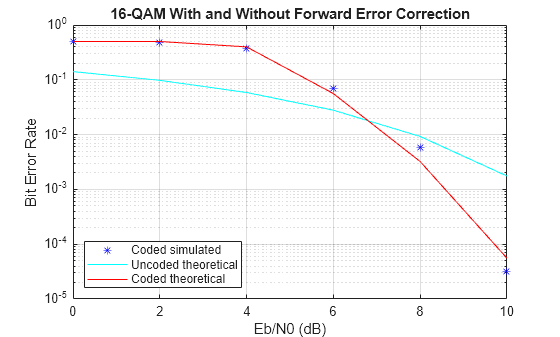
Plot BER versus curves for the simulated coded data, and the theoretical uncoded and coded data. At higher values, the error correcting code provides performance benefits. The simulated coded error rate results show good correlation to the theoretical coded results.
semilogy(ebnoVec,errorStats(:,1),'b*', ...
    ebnoVec,berUncoded_emp,'c-', ...
    ebnoVec,berCoded_emp,'r')
grid
legend('Coded simulated','Uncoded theoretical','Coded theoretical', ...
     'Location','southwest')
title('16-QAM With and Without Forward Error Correction')
xlabel('Eb/N0 (dB)')
ylabel('Bit Error Rate')