Sensitivity of Multiple Roots
This example shows that high-multiplicity poles have high numerical sensitivity and can shift by significant amounts when switching model representation.
Example
Poles with high multiplicity and clusters of nearby poles can be very sensitive to rounding errors, which can sometimes have dramatic consequences. This example uses a 15th-order discrete-time state-space model Hss with a cluster of stable poles near z=1:
load numdemo Hss
Convert the model to transfer function using tf:
Htf = tf(Hss);
Response Comparison
Compare the step responses of Hss and Htf to see how pole sensitivity can affect the stability of the model and cause large variations in the computed time and frequency responses:
step(Hss,'b',Htf,'r',20)
legend('Hss','Htf')

The step response of Htf diverges even though the state-space model Hss is stable (all its poles lie in the unit circle). The Bode plot also shows a large discrepancy between the state-space and transfer function models:
bode(Hss,'b',Htf,'r--')
legend('Hss','Htf')

The algorithm used to convert from state space to transfer function is not causing this discrepancy. If you convert from state space to zero-pole-gain, the first step in any SS to TF conversion, the discrepancies disappear:
Hzpk = zpk(Hss);

step(Hss,'b',Hzpk,'r--')
legend('Hss','Hzpk')

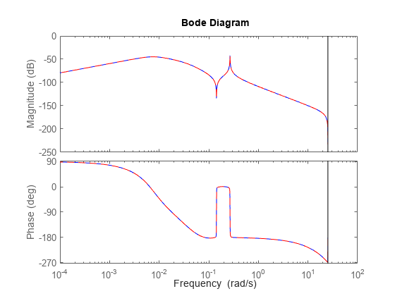
bode(Hss,'b',Hzpk,'r--')

This analysis shows that discrepancies arise in the ZPK to TF conversion, which merely involves computing a polynomial from its roots.
Cause of Discrepancy
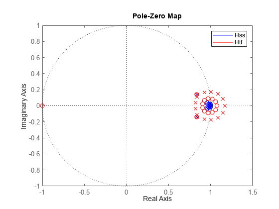
To understand the cause of these large discrepancies, compare the pole/zero maps of the state-space model and its transfer function:
pzplot(Hss,'b',Htf,'r')
legend('Hss','Htf')

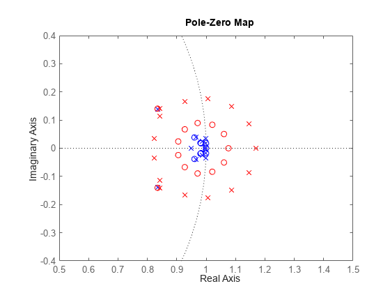
Note the tightly packed cluster of poles near z=1 in Hss. When these poles are recombined into the transfer function denominator, roundoff errors perturb the pole cluster into an evenly-distributed ring of poles around z=1 (a typical pattern for perturbed multiple roots). Unfortunately, some perturbed poles cross the unit circle and make the transfer function unstable. Zoom in on the plot to see these poles:
pzplot(Hss,'b',Htf,'r');
axis([0.5 1.5 -.4 .4])

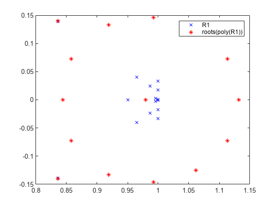
You can confirm this explanation with a simple experiment. Construct a polynomial whose roots are the poles R1 of Hss, compute the roots of this polynomial, and compare these roots with R1:
R1 = pole(Hss);                  % poles of Hss
Den = poly(R1);                  % polynomial with roots R1
R2 = roots(Den);                 % roots of this polynomial
plot(real(R1),imag(R1),'bx',real(R2),imag(R2),'r*')
legend('R1','roots(poly(R1))');

This plot shows that ROOTS(POLY(R1)) is quite different from R1 because of the clustered roots. As a result, the roots of the transfer function denominator differ significantly from the poles of the original state-space model Hss.
In conclusion, you should avoid converting state-space or zero-pole-gain models to transfer function form because this process can incur significant loss of accuracy.