Transient Goal

Purpose

Shape how the closed-loop system responds to a specific input signal when using Control System Tuner. Use a reference model to specify the desired transient response.

Description

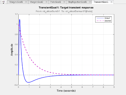
Transient Goal constrains the transient response from specified input locations to specified output locations. This requirement specifies that the transient response closely match the response of a reference model. The constraint is satisfied when the relative difference between the tuned and target responses falls within the tolerance you specify.

You can constrain the response to an impulse, step, or ramp input signal. You can also constrain the response to an input signal that is given by the impulse response of an input filter you specify.

Creation

In the Tuning tab of Control System Tuner, select New Goal > Transient response matching to create a Transient Goal.

Command-Line Equivalent

When tuning control systems at the command line, use TuningGoal.Transient to specify a step response goal.

Response Selection

Use this section of the dialog box to specify input, output, and loop-opening locations for evaluating the tuning goal.

Specify response inputs
Select one or more signal locations in your model at which to apply the input. To constrain a SISO response, select a single-valued input signal. For example, to constrain the transient response from a location named 'u' to a location named 'y', click Add signal to list and select 'u'. To constrain a MIMO response, select multiple signals or a vector-valued signal.
Specify response outputs
Select one or more signal locations in your model at which to measure the transient response. To constrain a SISO response, select a single-valued output signal. For example, to constrain the transient response from a location named 'u' to a location named 'y', click Add signal to list and select 'y'. To constrain a MIMO response, select multiple signals or a vector-valued signal. For MIMO systems, the number of outputs must equal the number of inputs.
Compute the response with the following loops open
Select one or more signal locations in your model at which to open a feedback loop for the purpose of evaluating this tuning goal. The tuning goal is evaluated against the open-loop configuration created by opening feedback loops at the locations you identify. For example, to evaluate the tuning goal with an opening at a location named 'x', click Add signal to list and select 'x'.

Tip

To highlight any selected signal in the Simulink^® model, click . To remove a signal from the input or output list, click . When you have selected multiple signals, you can reorder them using and . For more information on how to specify signal locations for a tuning goal, see Specify Goals for Interactive Tuning.

Initial Signal Selection

Select the input signal shape for the transient response you want to constrain in Control System Tuner.

Impulse — Constrain the response to a unit impulse.
Step — Constrain the response to a unit step. Using Step is equivalent to using a Step Tracking Goal.
Ramp — Constrain the response to a unit ramp, u = t.
Other — Constrain the response to a custom input signal. Specify the custom input signal by entering a transfer function (tf or zpkmodel) in the Use impulse response of filter field. The custom input signal is the response of this transfer function to a unit impulse.
This transfer function represents the Laplace transform of the desired custom input signal. For example, to constrain the transient response to a unit-amplitude sine wave of frequency w, enter tf(w,[1,0,w^2]). This transfer function is the Laplace transform of sin(wt).
The transfer function you enter must be continuous, and can have no poles in the open right-half plane. The series connection of this transfer function with the reference system for the desired transient response must have no feedthrough term.

Desired Transient Response

Specify the reference system for the desired transient response as a dynamic system model, such as a tf, zpk, or ss model. The Transient Goal constrains the system response to closely match the response of this system to the input signal you specify in Initial Signal Selection.

Enter the name of the reference model in the MATLAB^® workspace in the Reference Model field. Alternatively, enter a command to create a suitable reference model, such as tf(1,[1 1.414 1]). The reference model must be stable, and the series connection of the reference model with the input shaping filter must have no feedthrough term.

Options

Use this section of the dialog box to specify additional characteristics of the transient response goal.

Keep % mismatch below
Specify the relative matching error between the actual (tuned) transient response and the target response. Increase this value to loosen the matching tolerance. The relative matching error, e_rel, is defined as:
$gap = \frac{{‖ y (t) - y_{r e f} (t) ‖}_{2}}{{‖ y_{r e f (t r)} (t) ‖}_{2}} .$
y(t) – y_ref(t) is the response mismatch, and 1 – y_ref(tr)(t) is the transient portion of y_ref (deviation from steady-state value or trajectory). ${‖ \cdot ‖}_{2}$ denotes the signal energy (2-norm). The gap can be understood as the ratio of the root-mean-square (RMS) of the mismatch to the RMS of the reference transient.
Adjust for amplitude of input signals and Adjust for amplitude of output signals
For a MIMO tuning goal, when the choice of units results in a mix of small and large signals in different channels of the response, this option allows you to specify the relative amplitude of each entry in the vector-valued signals. This information is used to scale the off-diagonal terms in the transfer function from the tuning goal inputs to outputs. This scaling ensures that cross-couplings are measured relative to the amplitude of each reference signal.
When these options are set to No, the closed-loop transfer function being constrained is not scaled for relative signal amplitudes. When the choice of units results in a mix of small and large signals, using an unscaled transfer function can lead to poor tuning results. Set the option to Yes to provide the relative amplitudes of the input signals and output signals of your transfer function.
For example, suppose the tuning goal constrains a 2-input, 2-output transfer function. Suppose further that second input signal to the transfer function tends to be about 100 times greater than the first signal. In that case, select Yes and enter [1,100] in the Amplitudes of input signals text box.
Adjusting signal amplitude causes the tuning goal to be evaluated on the scaled transfer function D_o^–1T(s)D_i, where T(s) is the unscaled transfer function. D_o and D_i are diagonal matrices with the Amplitudes of output signals and Amplitudes of input signals values on the diagonal, respectively.
The default value, No, means no scaling is applied.
Apply goal to
Use this option when tuning multiple models at once, such as an array of models obtained by linearizing a Simulink model at different operating points or block-parameter values. By default, active tuning goals are enforced for all models. To enforce a tuning requirement for a subset of models in an array, select Only Models. Then, enter the array indices of the models for which the goal is enforced. For example, suppose you want to apply the tuning goal to the second, third, and fourth models in a model array. To restrict enforcement of the requirement, enter 2:4 in the Only Models text box.
For more information about tuning for multiple models, see Robust Tuning Approaches (Robust Control Toolbox).

Tips

When you use this requirement to tune a control system, Control System Tuner attempts to enforce zero feedthrough (D = 0) on the transfer that the requirement constrains. Zero feedthrough is imposed because the H₂ norm, and therefore the value of the tuning goal (see Algorithms), is infinite for continuous-time systems with nonzero feedthrough.
Control System Tuner enforces zero feedthrough by fixing to zero all tunable parameters that contribute to the feedthrough term. Control System Tuner returns an error when fixing these tunable parameters is insufficient to enforce zero feedthrough. In such cases, you must modify the requirement or the control structure, or manually fix some tunable parameters of your system to values that eliminate the feedthrough term.
When the constrained transfer function has several tunable blocks in series, the software’s approach of zeroing all parameters that contribute to the overall feedthrough might be conservative. In that case, it is sufficient to zero the feedthrough term of one of the blocks. If you want to control which block has feedthrough fixed to zero, you can manually fix the feedthrough of the tuned block of your choice.
To fix parameters of tunable blocks to specified values, see View and Change Block Parameterization in Control System Tuner.
This tuning goal also imposes an implicit stability constraint on the closed-loop transfer function between the specified inputs to outputs, evaluated with loops opened at the specified loop-opening locations. The dynamics affected by this implicit constraint are the stabilized dynamics for this tuning goal. The Minimum decay rate and Maximum natural frequency tuning options control the lower and upper bounds on these implicitly constrained dynamics. If the optimization fails to meet the default bounds, or if the default bounds conflict with other requirements, on the Tuning tab, use Tuning Options to change the defaults.

Algorithms

When you tune a control system, the software converts each tuning goal into a normalized scalar value f(x). Here, x is the vector of free (tunable) parameters in the control system. The software then adjusts the parameter values to minimize f(x) or to drive f(x) below 1 if the tuning requirement is a hard constraint.

For Transient Goal, f(x) is based upon the relative gap between the tuned response and the target response:

$gap = \frac{{‖ y (t) - y_{r e f} (t) ‖}_{2}}{{‖ y_{r e f (t r)} (t) ‖}_{2}} .$

y(t) – y_ref(t) is the response mismatch, and 1 – y_ref(tr)(t) is the transient portion of y_ref (deviation from steady-state value or trajectory). ${‖ \cdot ‖}_{2}$ denotes the signal energy (2-norm). The gap can be understood as the ratio of the root-mean-square (RMS) of the mismatch to the RMS of the reference transient.