Confidence and Prediction Bounds
About Confidence and Prediction Bounds
Curve Fitting Toolbox™ software lets you calculate confidence bounds for the fitted coefficients, and prediction bounds for new observations or for the fitted function. Additionally, for prediction bounds, you can calculate simultaneous bounds, which take into account all predictor values, or you can calculate nonsimultaneous bounds, which take into account only individual predictor values. The coefficient confidence bounds are presented numerically, while the prediction bounds are displayed graphically and are also available numerically.
The available confidence and prediction bounds are summarized below.
Types of Confidence and Prediction Bounds
Interval Type | Description |
|---|---|
Fitted coefficients | Confidence bounds for the fitted coefficients |
New observation | Prediction bounds for a new observation (response value) |
New function | Prediction bounds for a new function value |
Note
Prediction bounds are also often described as confidence bounds because you are calculating a confidence interval for a predicted response.
Confidence and prediction bounds define the lower and upper values of the associated interval, and define the width of the interval. The width of the interval indicates how uncertain you are about the fitted coefficients, the predicted observation, or the predicted fit. For example, a very wide interval for the fitted coefficients can indicate that you should use more data when fitting before you can say anything very definite about the coefficients.
The bounds are defined with a level of certainty that you specify. The level of certainty is often 95%, but it can be any value such as 90%, 99%, 99.9%, and so on. For example, you might want to take a 5% chance of being incorrect about predicting a new observation. Therefore, you would calculate a 95% prediction interval. This interval indicates that you have a 95% chance that the new observation is actually contained within the lower and upper prediction bounds.
Confidence Bounds on Coefficients
The confidence bounds for fitted coefficients are given by
where b are the coefficients produced by the fit, t depends on the confidence level, and is computed using the inverse of Student's t cumulative distribution function, and S is a vector of the diagonal elements from the estimated covariance matrix of the coefficient estimates, (XTX)–1s2. In a linear fit, X is the design matrix, while for a nonlinear fit X is the Jacobian of the fitted values with respect to the coefficients. XT is the transpose of X, and s2 is the mean squared error.
You can view the confidence bounds in the Curve Fitter app. The app displays the bounds in the Coefficients and 95% Confidence Bounds table in the Results pane.

The fitted value for the coefficient p1 is
-0.6675, the lower bound is -0.7622, and
the upper bound is -0.5728.
You can calculate confidence intervals at the command line with the confint function.
Prediction Bounds on Fits
As mentioned previously, you can calculate prediction bounds for the fitted curve. The prediction is based on an existing fit to the data. Additionally, the bounds can be simultaneous and measure the confidence for all predictor values, or they can be nonsimultaneous and measure the confidence only for a single predetermined predictor value. If you are predicting a new observation, nonsimultaneous bounds measure the confidence that the new observation lies within the interval given a single predictor value. Simultaneous bounds measure the confidence that a new observation lies within the interval regardless of the predictor value.
| Bound Type | Observation | Functional |
|---|---|---|
| Simultaneous |
|
|
| Nonsimultaneous |
|
|
Where:
s2 is the mean squared error
t depends on the confidence level, and is computed using the inverse of Student's t cumulative distribution function
f depends on the confidence level, and is computed using the inverse of the F cumulative distribution function.
S is the covariance matrix of the coefficient estimates, (XTX)–1s2.
x is a row vector of the design matrix or Jacobian evaluated at a specified predictor value.
You can graphically display prediction bounds using the Curve Fitter app. In the
Curve Fitter app, you can display nonsimultaneous prediction bounds for new
observations. On the Curve Fitter tab, in the
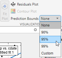
Visualization section, select a level of certainty from the
Prediction Bounds list. You can change this level to any
value by selecting Custom from the list.
You can display numerical prediction bounds of any type at the command line with
the predint function.
To understand the quantities associated with each type of prediction interval, recall that the data, fit, and residuals are related through the formula
data = fit + residuals
where the fit and residuals terms are estimates of terms in the formula
data = model + random error
Suppose you plan to take a new observation at the predictor value xn+1. Call the new observation yn+1(xn+1) and the associated error εn+1. Then
yn+1(xn+1) = f(xn+1) + εn+1
where f(xn+1) is the true but unknown function you want to estimate at xn+1. The likely values for the new observation or for the estimated function are provided by the nonsimultaneous prediction bounds.
If instead you want the likely value of the new observation to be associated with any predictor value, the previous equation becomes
yn+1(x) = f(x) + ε
The likely values for this new observation or for the estimated function are provided by the simultaneous prediction bounds.
The types of prediction bounds are summarized below.
Types of Prediction Bounds
Type of Bound | Simultaneous or Nonsimultaneous | Associated Equation |
|---|---|---|
Observation | Nonsimultaneous | yn+1(xn+1) |
Simultaneous | yn+1(x), for all x | |
Function | Nonsimultaneous | f(xn+1) |
Simultaneous | f(x), for all x |
The nonsimultaneous and simultaneous prediction bounds for a new observation and the fitted function are shown below. Each graph contains three curves: the fit, the lower confidence bounds, and the upper confidence bounds. The fit is a single-term exponential to generated data and the bounds reflect a 95% confidence level. Note that the intervals associated with a new observation are wider than the fitted function intervals because of the additional uncertainty in predicting a new response value (the curve plus random errors).

Calculate Prediction Intervals from the Command Line
Calculate and plot observation and functional prediction intervals for a fit to noisy data.
Generate noisy data with an exponential trend.
x = (0:0.2:5)';
y = 2*exp(-0.2*x) + 0.5*randn(size(x));
Fit a curve to the data using a single-term exponential.
fitresult = fit(x,y,'exp1');Compute 95% observation and functional prediction intervals, both simultaneous and nonsimultaneous. Nonsimultaneous bounds are for individual elements of x; simultaneous bounds are for all elements of x.
p11 = predint(fitresult,x,0.95,'observation','off');
p12 = predint(fitresult,x,0.95,'observation','on');
p21 = predint(fitresult,x,0.95,'functional','off');
p22 = predint(fitresult,x,0.95,'functional','on');
Plot the data, fit, and prediction intervals. Observation bounds are wider than functional bounds because they measure the uncertainty of predicting the fitted curve plus the random variation in the new observation.
subplot(2,2,1)
plot(fitresult,x,y), hold on, plot(x,p11,'m--'), xlim([0 5]), ylim([-1 5])
title('Nonsimultaneous Observation Bounds','FontSize',9)
legend off

subplot(2,2,2)
plot(fitresult,x,y), hold on, plot(x,p12,'m--'), xlim([0 5]), ylim([-1 5])
title('Simultaneous Observation Bounds','FontSize',9)
legend off

subplot(2,2,3)
plot(fitresult,x,y), hold on, plot(x,p21,'m--'), xlim([0 5]), ylim([-1 5])
title('Nonsimultaneous Functional Bounds','FontSize',9)
legend off

subplot(2,2,4)
plot(fitresult,x,y), hold on, plot(x,p22,'m--'), xlim([0 5]), ylim([-1 5])
title('Simultaneous Functional Bounds','FontSize',9)
legend({'Data','Fitted curve', 'Prediction intervals'},...
       'FontSize',8,'Location','northeast')

Calculate Prediction Bounds Using Curve Fitter App
Load the census data set.
load censusThe variables cdate and pop contain data for the date and population when the census was taken.
Open the Curve Fitter app.
curveFitter
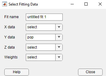
In the app, select the data variables for the fit. On the Curve Fitter tab, in the Data section, click Select Data. In the Select Fitting Data dialog box, select cdate as the X data value and pop as the Y data value.

The app plots the data points as you select the variables.

The plot shows the census data and the linear fit for the data.
Plot the 95% prediction bounds for the fit. In the Visualization section of the Curve Fitter tab, select 95% for Prediction Bounds.


The plot now shows the 95% prediction intervals in addition to the census data and linear fit.
To plot the 60% prediction bounds for the fit, you must specify a custom confidence level. In the Visualization section of the Curve Fitter tab, select Custom for Prediction Bounds. In the Set Prediction Bounds dialog box, type 60 in Confidence level (%) box, and click OK.


The plot now shows the 60% prediction intervals in addition to the census data and linear fit. Together, the two plots show that the 60% prediction intervals lie closer to the linear fit than the 95% prediction intervals.