Long Short-Term Memory Neural Networks
This topic explains how to work with sequence and time series data for classification and regression tasks using long short-term memory (LSTM) neural networks. For an example showing how to classify sequence data using an LSTM neural network, see Sequence Classification Using Deep Learning.
An LSTM neural network is a type of recurrent neural network (RNN) that can learn long-term dependencies between time steps of sequence data.
LSTM Neural Network Architecture
The core components of an LSTM neural network are a sequence input layer and an LSTM layer. A sequence input layer inputs sequence or time series data into the neural network. An LSTM layer learns long-term dependencies between time steps of sequence data.
This diagram illustrates the architecture of a simple LSTM neural network for classification. The neural network starts with a sequence input layer followed by an LSTM layer. To predict class labels, the neural network ends with a fully connected layer, and a softmax layer.

This diagram illustrates the architecture of a simple LSTM neural network for regression. The neural network starts with a sequence input layer followed by an LSTM layer. The neural network ends with a fully connected layer.

Classification LSTM Networks
To create an LSTM network for sequence-to-label classification, create a layer array containing a sequence input layer, an LSTM layer, a fully connected layer, and a softmax layer.
Set the size of the sequence input layer to the number of features of the input data. Set the size of the fully connected layer to the number of classes. You do not need to specify the sequence length.
For the LSTM layer, specify the number of hidden units and the output mode "last".
numFeatures = 12;
numHiddenUnits = 100;
numClasses = 9;
layers = [ ...
    sequenceInputLayer(numFeatures)
    lstmLayer(numHiddenUnits,OutputMode="last")
    fullyConnectedLayer(numClasses)
    softmaxLayer];
For an example showing how to train an LSTM network for sequence-to-label classification and classify new data, see Sequence Classification Using Deep Learning.
To create an LSTM network for sequence-to-sequence classification, use the same architecture as for sequence-to-label classification, but set the output mode of the LSTM layer to "sequence".
numFeatures = 12;
numHiddenUnits = 100;
numClasses = 9;
layers = [ ...
    sequenceInputLayer(numFeatures)
    lstmLayer(numHiddenUnits,OutputMode="sequence")
    fullyConnectedLayer(numClasses)
    softmaxLayer];
Regression LSTM Networks
To create an LSTM network for sequence-to-one regression, create a layer array containing a sequence input layer, an LSTM layer, and a fully connected layer.
Set the size of the sequence input layer to the number of features of the input data. Set the size of the fully connected layer to the number of responses. You do not need to specify the sequence length.
When you train the neural network, you can automatically normalize the training targets using the NormalizeTargets training option (introduced in R2026a). Using normalized targets helps stabilize training and results in training predictions that closely match the normalized targets. To make the neural network output predictions in the space of unnormalized values at prediction time only, include an inverse normalization layer (introduced in R2026a). Before R2026a: To stabilize training, normalize the targets manually before you train the neural network.
For the LSTM layer, specify the number of hidden units and the output mode "last".
numFeatures = 12;
numHiddenUnits = 125;
numResponses = 1;

layers = [ ...
    sequenceInputLayer(numFeatures)
    lstmLayer(numHiddenUnits,OutputMode="last")
    fullyConnectedLayer(numResponses)
    inverseNormalizationLayer];
To create an LSTM network for sequence-to-sequence regression, use the same architecture as for sequence-to-one regression, but set the output mode of the LSTM layer to "sequence".
numFeatures = 12;
numHiddenUnits = 125;
numResponses = 1;

layers = [ ...
    sequenceInputLayer(numFeatures)
    lstmLayer(numHiddenUnits,OutputMode="sequence")
    fullyConnectedLayer(numResponses)
    inverseNormalizationLayer];
For an example showing how to train an LSTM network for sequence-to-sequence regression and predict on new data, see Sequence-to-Sequence Regression Using Deep Learning.
Video Classification Network
To create a deep learning network for data containing sequences of images such as video data and medical images, specify image sequence input using the sequence input layer.
Specify the layers and create a dlnetwork object.
inputSize = [64 64 3];
filterSize = 5;
numFilters = 20;
numHiddenUnits = 200;
numClasses = 10;

layers = [
    sequenceInputLayer(inputSize)
    convolution2dLayer(filterSize,numFilters)
    batchNormalizationLayer
    reluLayer
    lstmLayer(numHiddenUnits,OutputMode="last")
    fullyConnectedLayer(numClasses)
    softmaxLayer];

net = dlnetwork(layers);
For an example showing how to train a deep learning network for video classification, see Classify Videos Using Deep Learning.
Deeper LSTM Networks
You can make LSTM networks deeper by inserting extra LSTM layers with the output mode "sequence" before the LSTM layer. To prevent overfitting, you can insert dropout layers after the LSTM layers.
For sequence-to-label classification networks, the output mode of the last LSTM layer must be "last".
numFeatures = 12;
numHiddenUnits1 = 125;
numHiddenUnits2 = 100;
numClasses = 9;
layers = [ ...
    sequenceInputLayer(numFeatures)
    lstmLayer(numHiddenUnits1,OutputMode="sequence")
    dropoutLayer(0.2)
    lstmLayer(numHiddenUnits2,OutputMode="last")
    dropoutLayer(0.2)
    fullyConnectedLayer(numClasses)
    softmaxLayer];
For sequence-to-sequence classification networks, the output mode of the last LSTM layer must be "sequence".
numFeatures = 12;
numHiddenUnits1 = 125;
numHiddenUnits2 = 100;
numClasses = 9;
layers = [ ...
    sequenceInputLayer(numFeatures)
    lstmLayer(numHiddenUnits1,OutputMode="sequence")
    dropoutLayer(0.2)
    lstmLayer(numHiddenUnits2,OutputMode="sequence")
    dropoutLayer(0.2)
    fullyConnectedLayer(numClasses)
    softmaxLayer];
Layers
| Icon | Layer | Description |
|---|---|---|
| A sequence input layer inputs sequence data to a neural network and applies data normalization. | |
| An embedding layer converts numeric indices to numeric vectors, where the indices correspond to discrete data. | |
| An LSTM layer is an RNN layer that learns long-term dependencies between time steps in time-series and sequence data. | ||
| An LSTM projected layer is an RNN layer that learns long-term dependencies between time steps in time-series and sequence data using projected learnable weights. | ||
| A bidirectional LSTM (BiLSTM) layer is an RNN layer that learns bidirectional long-term dependencies between time steps of time-series or sequence data. These dependencies can be useful when you want the RNN to learn from the complete time series at each time step. | ||
| A GRU layer is an RNN layer that learns dependencies between time steps in time-series and sequence data. | ||
| A GRU projected layer is an RNN layer that learns dependencies between time steps in time-series and sequence data using projected learnable weights. | ||
| A 1-D convolutional layer applies sliding convolutional filters to 1-D input. | ||
| A transposed 1-D convolution layer upsamples one-dimensional feature maps. | ||
| A 1-D max pooling layer performs downsampling by dividing the input into 1-D pooling regions, then computing the maximum of each region. | ||
| A 1-D average pooling layer performs downsampling by dividing the input into 1-D pooling regions, then computing the average of each region. | ||
| A 1-D global max pooling layer performs downsampling by outputting the maximum of the time or spatial dimensions of the input. | ||
| A flatten layer collapses the spatial dimensions of the input into the channel dimension. | ||
| A word embedding layer maps word indices to vectors. | |
| A peephole LSTM layer is a variant of an LSTM layer, where the gate calculations use the layer cell state. |
Classification, Prediction, and Forecasting
To make predictions on new data, use the minibatchpredict function. To
convert predicted classification scores to labels, use the scores2label.
LSTM neural networks can remember the state of the neural network between predictions. The RNN state is useful when you do not have the complete time series in advance, or if you want to make multiple predictions on a long time series.
To predict and classify on parts of a time series and update the RNN state, use the
predict function and
also return and update the neural network state. To reset the RNN state between
predictions, use resetState.
For an example showing how to forecast future time steps of a sequence, see Time Series Forecasting Using Deep Learning.
Sequence Padding and Truncation
LSTM neural networks support input data with varying sequence lengths. When passing
data through the neural network, the software pads or truncates sequences so that all
the sequences in each mini-batch have the specified length. You can specify the sequence
lengths and the value used to pad the sequences using the SequenceLength and SequencePaddingValue training options.
After training the neural network, you can use the same mini-batch size and padding
options when you use the minibatchpredict function.
Sort Sequences by Length
To reduce the amount of padding or discarded data when padding or truncating
sequences, try sorting your data by sequence length. For sequences where the first
dimension corresponds to the time steps, to sort the data by sequence length, first
get the number of columns of each sequence by applying size(X,1)
to every sequence using cellfun. Then sort the sequence lengths
using sort, and use the second output to reorder the original
sequences.
sequenceLengths = cellfun(@(X) size(X,1), XTrain);
[sequenceLengthsSorted,idx] = sort(sequenceLengths);
XTrain = XTrain(idx);

Pad Sequences
If the SequenceLength training or prediction option is
"longest", then the software pads the sequences so that all
the sequences in a mini-batch have the same length as the longest sequence in the
mini-batch. This option is the default.

Truncate Sequences
If the SequenceLength training or prediction option is
"shortest", then the software truncates the sequences so that
all the sequences in a mini-batch have the same length as the shortest sequence in
that mini-batch. The remaining data in the sequences is discarded.

Specify Padding Direction
The location of the padding and
truncation can impact training, classification, and prediction accuracy. Try setting
the SequencePaddingDirection training options to
"left" or "right" and see which is best
for your data.
Recurrent layers process sequence data one time step at a time, so when the recurrent layer
OutputMode property is "last", any padding in the
final time steps can negatively influence the layer output. To pad or truncate sequence data
on the left, set the SequencePaddingDirection name-value argument to
"left".
For sequence-to-sequence neural networks (when the OutputMode property is
"sequence" for each recurrent layer), any padding in the first time
steps can negatively influence the predictions for the earlier time steps. To pad or
truncate sequence data on the right, set the SequencePaddingDirection name-value argument to "right".


Normalize Sequence Data
To recenter training data automatically at training time using zero-center
normalization, set the Normalization option of sequenceInputLayer to
"zerocenter". Alternatively, you can normalize sequence data by
first calculating the per-feature mean and standard deviation of all the sequences.
Then, for each training observation, subtract the mean value and divide by the standard
deviation.
mu = mean([XTrain{:}],1);
sigma = std([XTrain{:}],0,1);
XTrain = cellfun(@(X) (X-mu)./sigma,XTrain,UniformOutput=false);
Out-of-Memory Data
Use datastores for sequence, time series, and signal data when data is too large to fit in memory or to perform specific operations when reading batches of data.
To learn more, see Train Network Using Out-of-Memory Sequence Data and Classify Out-of-Memory Text Data Using Deep Learning.
Visualization
Investigate and visualize the features
learned by LSTM neural networks from sequence and time series data by extracting the
activations using the minibatchpredict function and setting the Outputs
argument. To learn more, see Visualize Activations of LSTM Network.
LSTM Layer Architecture
This diagram illustrates the flow of data through an LSTM layer with input and output with T time steps. In the diagram, denotes the output (also known as the hidden state) and denotes the cell state at time step t.
If the layer outputs the full sequence, then it outputs , …, , which is equivalent to , …, . If the layer outputs the last time step only, then the layer outputs , which is equivalent to . The number of channels in the output matches the number of hidden units of the LSTM layer.
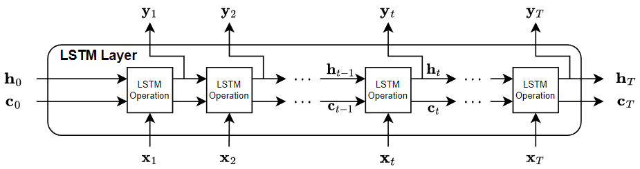
The first LSTM operation uses the initial state of the RNN and the first time step of the sequence to compute the first output and the updated cell state. At time step t, the operation uses the current state of the RNN and the next time step of the sequence to compute the output and the updated cell state .
The state of the layer consists of the hidden state (also known as the output state) and the cell state. The hidden state at time step t contains the output of the LSTM layer for this time step. The cell state contains information learned from the previous time steps. At each time step, the layer adds information to or removes information from the cell state. The layer controls these updates using gates.
These components control the cell state and hidden state of the layer.
| Component | Purpose |
|---|---|
| Input gate (i) | Control level of cell state update |
| Forget gate (f) | Control level of cell state reset (forget) |
| Cell candidate (g) | Add information to cell state |
| Output gate (o) | Control level of cell state added to hidden state |
This diagram illustrates the flow of data at time step t. This diagram shows how the gates forget, update, and output the cell and hidden states.

The learnable weights of an LSTM layer are the input weights W
(InputWeights), the recurrent weights R
(RecurrentWeights), and the bias b
(Bias). The matrices W, R,
and b are concatenations of the input weights, the recurrent weights, and
the bias of each component, respectively. The layer concatenates the matrices according to
these equations:
where i, f, g, and o denote the input gate, forget gate, cell candidate, and output gate, respectively.
The cell state at time step t is given by
where denotes the Hadamard product (element-wise multiplication of vectors).
The hidden state at time step t is given by
where denotes the state activation function. By default, the
lstmLayer function uses the hyperbolic tangent function (tanh) to
compute the state activation function.
These formulas describe the components at time step t.
| Component | Formula |
|---|---|
| Input gate | |
| Forget gate | |
| Cell candidate | |
| Output gate |
In these calculations, denotes the gate activation function. By default, the
lstmLayer function, uses the sigmoid function, given by , to compute the gate activation function.
References
[1] Hochreiter, S., and J. Schmidhuber. "Long short-term memory." Neural computation. Vol. 9, Number 8, 1997, pp.1735–1780.
See Also
sequenceInputLayer | lstmLayer | bilstmLayer | gruLayer | dlnetwork | minibatchpredict | predict | scores2label | flattenLayer | wordEmbeddingLayer (Text Analytics Toolbox)
Topics
- Sequence Classification Using Deep Learning
- Time Series Forecasting Using Deep Learning
- Sequence-to-Sequence Classification Using Deep Learning
- Sequence-to-Sequence Regression Using Deep Learning
- Sequence-to-One Regression Using Deep Learning
- Classify Videos Using Deep Learning
- Visualize Activations of LSTM Network
- Develop Custom Mini-Batch Datastore
- Example Deep Learning Network Architectures
- Deep Learning in MATLAB