Sequence-to-Sequence Regression Using Deep Learning

This example shows how to predict the remaining useful life (RUL) of engines by using deep learning.

To train a deep neural network to predict numeric values from time series or sequence data, you can use a long short-term memory (LSTM) network.

This example uses the Turbofan Engine Degradation Simulation Data Set as described in [1]. The example trains an LSTM network to predict the remaining useful life of an engine (predictive maintenance), measured in cycles, given time series data representing various sensors in the engine. The training data contains simulated time series data for 100 engines. Each sequence varies in length and corresponds to a full run to failure (RTF) instance. The test data contains 100 partial sequences and corresponding values of the remaining useful life at the end of each sequence.

The data set contains 100 training observations and 100 test observations.

Download Data

Download and unzip the Turbofan Engine Degradation Simulation data set.

Each time series of the Turbofan Engine Degradation Simulation data set represents a different engine. Each engine starts with unknown degrees of initial wear and manufacturing variation. The engine is operating normally at the start of each time series, and develops a fault at some point during the series. In the training set, the fault grows in magnitude until system failure.

The data contains a ZIP-compressed text files with 26 columns of numbers, separated by spaces. Each row is a snapshot of data taken during a single operational cycle, and each column is a different variable. The columns correspond to the following:

Column 1 – Unit number
Column 2 – Time in cycles
Columns 3–5 – Operational settings
Columns 6–26 – Sensor measurements 1–21

Create a directory to store the Turbofan Engine Degradation Simulation data set.

dataFolder = fullfile(tempdir,"turbofan");
if ~exist(dataFolder,"dir")
    mkdir(dataFolder);
end

Download and extract the Turbofan Engine Degradation Simulation data set.

filename = matlab.internal.examples.downloadSupportFile("nnet","data/TurbofanEngineDegradationSimulationData.zip");
unzip(filename,dataFolder)

Prepare Training Data

Load the data using the function processTurboFanDataTrain attached to this example. The function processTurboFanDataTrain extracts the data from filenamePredictors and returns the cell arrays XTrain and TTrain, which contain the training predictor and response sequences.

filenamePredictors = fullfile(dataFolder,"train_FD001.txt");
[XTrain,TTrain] = processTurboFanDataTrain(filenamePredictors);

Remove Features with Constant Values

Features that remain constant for all time steps can negatively impact the training. Find the columns of data that have the same minimum and maximum values, and remove them.

XTrainConcatenatedTimesteps = cat(1,XTrain{:});
m = min(XTrainConcatenatedTimesteps,[],1);
M = max(XTrainConcatenatedTimesteps,[],1);
idxConstant = M == m;

for i = 1:numel(XTrain)
    XTrain{i}(:,idxConstant) = [];
end

View the number of remaining features in the sequences.

numFeatures = size(XTrain{1},2)

numFeatures = 
17

Calculate Normalization Statistics

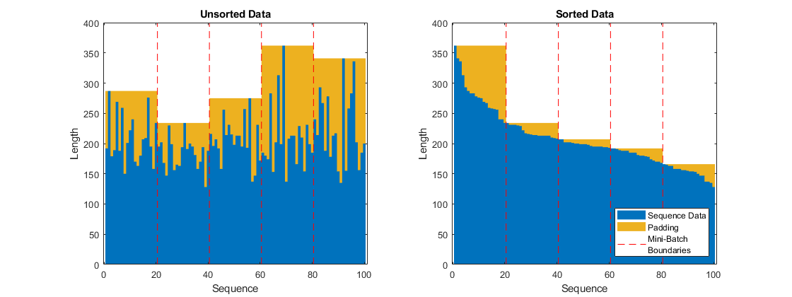
The neural network in this example uses a sequence input layer, which supports normalizing the input data using automatically calculated normalization statistics. Because the training sequences used in this example have different lengths, the software zero-pads them so that the sequences in each mini-batch have the same length. The zero-valued elements that correspond to padding can negatively impact the calculation of the normalization statistics, so compute the statistics manually instead.

To calculate the mean and standard deviation over all observations, concatenate the sequence data horizontally.

XTrainConcatenatedTimesteps = cat(1,XTrain{:});
mu = mean(XTrainConcatenatedTimesteps,1);
sig = std(XTrainConcatenatedTimesteps,0,1);

Clip Responses

To learn more from the sequence data when the engines are close to failing, clip the responses at the threshold 150. This makes the network treat instances with higher RUL values as equal.

thr = 150;
for i = 1:numel(TTrain)
    TTrain{i}(TTrain{i} > thr) = thr;
end

This figure shows the first observation and the corresponding clipped response.

Define Network Architecture

Define the network architecture:

Specify a sequence input layer that applies $Z$ -score normalization using the manually computed normalization statistics.
For the LSTM layer, specify 200 hidden units.
Include fully connected layer with an output size of 50 followed by a dropout layer with dropout probability 0.5.
For regression, include a fully connected layer with an output size that matches the number of responses.
In this example, the training process automatically normalizes the training targets using the NormalizeTargets training option (introduced in R2026a). Using normalized targets helps stabilize training and results in training predictions that closely match the normalized targets. To make the neural network output predictions in the space of unnormalized values at prediction time only, include an inverse normalization layer (introduced in R2026a) that applies the inverse symmetric rescaling operation. Before R2026a: To stabilize training, normalize the targets manually before you train the neural network.

numHiddenUnits = 200;
fcOutputSize = 50;
dropoutProbability = 0.5;

numResponses = size(TTrain{1},2);

layers = [ ...
    sequenceInputLayer(numFeatures,Normalization="zscore",Mean=mu',StandardDeviation=sig')
    lstmLayer(numHiddenUnits,OutputMode="sequence")
    fullyConnectedLayer(fcOutputSize)
    dropoutLayer(dropoutProbability)
    fullyConnectedLayer(numResponses)
    inverseNormalizationLayer(Normalization="rescale-symmetric")];

Because the targets have a lower limit of 0 and an upper limit of the clipping threshold, target values introduced by zero-padding do not affect the target normalization statistics used for rescaling.

Specify Training Options

Specify the training options. Choosing among the options requires empirical analysis. To explore different training option configurations by running experiments, you can use the Experiment Manager app.

Train using the Adam solver.
Automatically normalize the training targets using the NormalizeTargets argument (introduced in R2026a). Before R2026a: To stabilize training, normalize the targets manually before you train the neural network.
Do not reset the normalization statistics of the input layer.
Left-pad the sequences.
Train for 80 epochs with mini-batches of size 20.
To prevent the gradients from exploding, set the gradient threshold to 1.
Shuffle the sequences every epoch.
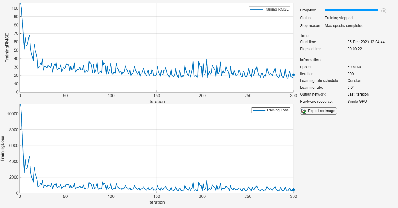
Display the training progress in a plot and monitor the root mean squared error (RMSE) metric.
Disable the verbose output.

maxEpochs = 80;
miniBatchSize = 20;

options = trainingOptions("adam", ...
    NormalizeTargets=true, ...
    ResetInputNormalization=false, ...
    SequencePaddingDirection="left", ...
    MaxEpochs=maxEpochs, ...
    MiniBatchSize=miniBatchSize, ...
    GradientThreshold=1, ...
    Shuffle="every-epoch", ...
    Plots="training-progress", ...
    Metrics="rmse", ...
    Verbose=false);

Train Neural Network

Train the neural network using the trainnet function. For regression, use mean squared error (MSE) loss. By default, the trainnet function uses a GPU if one is available. Using a GPU requires a Parallel Computing Toolbox™ license and a supported GPU device. For information on supported devices, see GPU Computing Requirements (Parallel Computing Toolbox). Otherwise, the function uses the CPU. To select the execution environment manually, use the ExecutionEnvironment training option.

net = trainnet(XTrain,TTrain,layers,"mse",options);

Test Neural Network

Prepare the test data using the function processTurboFanDataTest attached to this example. The function processTurboFanDataTest extracts the data from filenamePredictors and filenameResponses and returns the cell arrays XTest and TTest, which contain the test predictor and response sequences, respectively.

filenamePredictors = fullfile(dataFolder,"test_FD001.txt");
filenameResponses = fullfile(dataFolder,"RUL_FD001.txt");
[XTest,TTest] = processTurboFanDataTest(filenamePredictors,filenameResponses);

Remove features with constant values using idxConstant calculated from the training data. Clip the test responses at the same threshold used for the training data.

for i = 1:numel(XTest)
    XTest{i}(:,idxConstant) = [];
    TTest{i}(TTest{i} > thr) = thr;
end

Make predictions using the neural network. To make predictions with multiple observations, use the minibatchpredict function. The minibatchpredict function automatically uses a GPU if one is available. Using a GPU requires a Parallel Computing Toolbox™ license and a supported GPU device. For information on supported devices, see GPU Computing Requirements. Otherwise, the function uses the CPU. To prevent the function from adding padding to the data, specify the mini-batch size 1. To return predictions in a cell array, set UniformOutput to false.

YTest = minibatchpredict(net,XTest, ...
    MiniBatchSize=1, ...
    UniformOutput=false);

The LSTM network makes predictions on the partial sequence one time step at a time. At each time step, the network predicts using the value at this time step, and the network state calculated from the previous time steps only. The network updates its state between each prediction. The minibatchpredict function returns a sequence of these predictions. The last element of the prediction corresponds to the predicted RUL for the partial sequence.

Alternatively, you can make predictions one time step at a time by using predict and updating the network State property. This is useful when you have the values of the time steps arriving in a stream. Usually, it is faster to make predictions on full sequences when compared to making predictions one time step at a time. For an example showing how to forecast future time steps by updating the network between single time step predictions, see Time Series Forecasting Using Deep Learning.

Visualize some of the predictions in a plot.

idx = randperm(numel(YTest),4);
figure
for i = 1:numel(idx)
    subplot(2,2,i)
    
    plot(TTest{idx(i)},"--")
    hold on
    plot(YTest{idx(i)},".-")
    hold off
    
    ylim([0 thr + 25])
    title("Test Observation " + idx(i))
    xlabel("Time Step")
    ylabel("RUL")
end
legend(["Test Data" "Predicted"],Location="southeast")

For a given partial sequence, the predicted current RUL is the last element of the predicted sequences. Calculate the RMSE of the predictions and visualize the prediction error in a histogram.

for i = 1:numel(TTest)
    TTestLast(i) = TTest{i}(end);
    YTestLast(i) = YTest{i}(end);
end
figure
err = sqrt(mean((YTestLast - TTestLast).^2))

err = single

24.9944

histogram(YTestLast - TTestLast)
title("RMSE = " + err)
ylabel("Frequency")
xlabel("Error")

References

Saxena, Abhinav, Kai Goebel, Don Simon, and Neil Eklund. "Damage propagation modeling for aircraft engine run-to-failure simulation." In Prognostics and Health Management, 2008. PHM 2008. International Conference on, pp. 1-9. IEEE, 2008.