smoothTrajectory

Create smooth, jerk-limited actor trajectory in driving scenario

Since R2021a

Syntax

smoothTrajectory(ac,waypoints)

smoothTrajectory(ac,waypoints,speed)

smoothTrajectory(ac,waypoints,speed,waittime)

smoothTrajectory(___,Name=Value)

smoothTrajectory(ac,waypoints,TimeOfArrival=timeOfArrival)

smoothTrajectory(ac,waypoints,TimeOfArrival=timeOfArrival,Name=Value)

Description

The smoothTrajectory function creates a smooth, jerk-limited trajectory for an actor in a driving scenario based on either the speed values or arrival times of an actor at each waypoint. The generated trajectory features a smooth transition of accelerations between waypoints, making it compatible for generating synthetic inertial navigation system (INS) and global navigation satellite system (GNSS) measurements from an insSensor System object™. For more details on how smoothTrajectory generates trajectories, see Algorithms. By default, the function creates a trajectory for a vehicle whose steering location is at its rear axle. To create a trajectory for a vehicle whose steering location is at its front axle, use the ReferenceSteerPosition name-value argument.

Smoothed Trajectory from Actor Speed Information

smoothTrajectory(ac,waypoints) creates a smooth trajectory for an actor or vehicle, ac, to follow from a set of waypoints. The actor travels at a constant speed of 30 meters per second.

smoothTrajectory(ac,waypoints,speed) also specifies the speed at which the actor or vehicle travels along the trajectory, in either forward or reverse motion.

smoothTrajectory(ac,waypoints,speed,waittime) also specifies wait times for an actor or vehicle. Use this syntax to pause the actor or vehicle at specific waypoints.

smoothTrajectory(___,Name=Value) specifies options using one or more name-value arguments in addition to any combination of arguments from the previous syntaxes. For example, Course=course specifies the course angle course, which defines the steering direction of the actor or vehicle at each waypoint.

Smoothed Trajectory from Actor Arrival Times

Since R2024b

smoothTrajectory(ac,waypoints,TimeOfArrival=timeOfArrival) creates a smoothed trajectory for an actor or vehicle, ac, from a set of waypoints, waypoints, using the arrival time of the actor at each waypoint timeOfArrival.

smoothTrajectory(ac,waypoints,TimeOfArrival=timeOfArrival,Name=Value) specifies options using one or more name-value arguments. For example, MotionDirection=motionDirection specifies the direction motionDirection for the actor to move at each waypoint.

Examples

Create Trajectory with Varying Speeds

Create a driving scenario containing a curved two-lane road.

scenario = drivingScenario('SampleTime',0.05);
roadcenters = [0 0; 24.2 27.7; 50 30];
lspec = lanespec(2);
road(scenario,roadcenters,'Lanes',lspec);

Add a vehicle to the scenario. Set a trajectory in which the vehicle slows down as it enters the curve.

v = vehicle(scenario,'ClassID',1);
waypoints = [2.6 1.0; 23.6 24.9; 45.5 28.6];
speed = [9 8 9];
smoothTrajectory(v,waypoints,speed)

Plot the scenario and run the simulation.

plot(scenario,'Waypoints','on','RoadCenters','on')
while advance(scenario)
    pause(scenario.SampleTime)
end

Create Trajectory with Wait Time at Intersection

Create a driving scenario containing a four-way intersection.

scenario = drivingScenario('SampleTime',0.02,'StopTime',20);

roadCenters = [0 0; 50 0];
laneSpecification = lanespec([1 1]);
road(scenario,roadCenters,'Lanes',laneSpecification);

roadCenters = [25 25; 25 -25];
road(scenario,roadCenters,'Lanes',laneSpecification);

Add the ego vehicle, which travels north but waits for one second at the intersection.

ego = vehicle(scenario,'ClassID',1,'Position',[2 -2 0]);
waypoints = [2 -2; 17.5 -2; 45 -2];
speed = [5 0 5];
waittime = [0 1 0];
smoothTrajectory(ego,waypoints,speed,waittime);

Add a bicyclist that travels east through the intersection at a constant speed without stopping.

bicycle = actor(scenario, ...
    'ClassID',3, ...
    'Length',1.7, ...
    'Width',0.45, ...
    'Height',1.7, ...
    'Position',[23 23 0]);
waypoints = [23 23; 23 -23];
speed = 4;
smoothTrajectory(bicycle,waypoints,speed);

Plot the scenario. The vehicle stops at the intersection for one second, then resumes driving after the bicyclist crosses the intersection.

plot(scenario)
while advance(scenario)
    pause(scenario.SampleTime)
end

Simulate Car Backing into Parking Space

Simulate a driving scenario in which a car drives in reverse to back into a parking space.

Create a driving scenario containing a parking lot.

scenario = drivingScenario;
vertices = [0 9; 18 9; 18 -9; 0 -9];
parkingLot(scenario,vertices,ParkingSpace=parkingSpace);

Create a car and define its trajectory. The car drives forward, stops, and then drives in reverse to back into the parking space. As the car enters the parking space, it has a yaw orientation angle that is 90 degrees counterclockwise from where it started.

car = vehicle(scenario,ClassID=1);
waypoints = [9 -5; 9 5; 6 -1.3; 2 -1.3];
speed = [3; 0; -2; 0];
yaw = [90 90 180 180];
smoothTrajectory(car,waypoints,speed,Yaw=yaw)

Plot the driving scenario and display the waypoints of the trajectory.

plot(scenario,Waypoints="on")
while advance(scenario)
    pause(scenario.SampleTime)
end

Create Pedestrian Trajectory

Create the trajectory of a pedestrian who takes a sharp right turn at an intersection.

Create a driving scenario. Add road segments that define an intersection.

scenario = drivingScenario;
roadCenters = [0 10; 0 -10];
road(scenario,roadCenters);
road(scenario,flip(roadCenters,2));

Add a pedestrian actor to the scenario.

pedestrian = actor(scenario, ...
    'ClassID',4, ...
    'Length',0.24, ...
    'Width',0.45, ...
    'Height',1.7, ...
    'Position',[-9 0 0], ...
    'RCSPattern',[-8 -8; -8 -8], ...
    'Mesh',driving.scenario.pedestrianMesh, ...
    'Name','Pedestrian');

Define the trajectory of the pedestrian. The pedestrian approaches the intersection, pauses briefly, and then takes a sharp right turn at the intersection. To define the sharp right turn, specify two waypoints at the intersection that are close together. For these waypoints, specify the yaw orientation angle of the second waypoint at a 90-degree angle from the first waypoint.

waypoints = [-9 0; -0.25 0; 0 -0.25; 0 -9];
speed = [1.5; 0; 0.5; 1.5];
yaw =  [0; 0; -90; -90];
waittime = [0; 0.2; 0; 0];
smoothTrajectory(pedestrian,waypoints,speed,waittime,'Yaw',yaw);

Plot the driving scenario and display the waypoints of the pedestrian.

plot(scenario,'Waypoints','on')
while advance(scenario)
    pause(0.001)
end

Generate INS Measurements from Driving Scenario

Generate measurements from an INS sensor that is mounted to a vehicle in a driving scenario. Plot the INS measurements against the ground truth state of the vehicle and visualize the velocity and acceleration profile of the vehicle.

Create Driving Scenario

Load the geographic data for a driving route at the MathWorks® Apple Hill campus in Natick, MA.

data = load('ahroute.mat');
latIn = data.latitude;
lonIn = data.longitude;

Convert the latitude and longitude coordinates of the route to Cartesian coordinates. Set the origin to the first coordinate in the driving route. For simplicity, assume an altitude of 0 for the route.

alt = 0;
origin = [latIn(1),lonIn(1),alt];
[xEast,yNorth,zUp] = latlon2local(latIn,lonIn,alt,origin);

Create a driving scenario. Set the origin of the converted route as the geographic reference point.

scenario = drivingScenario('GeoReference',origin);

Create a road based on the Cartesian coordinates of the route.

roadCenters = [xEast,yNorth,zUp];
road(scenario,roadCenters);

Create a vehicle that follows the center line of the road. The vehicle travels between 4 and 5 meters per second (9 to 11 miles per hour), slowing down at the curves in the road. To create the trajectory, use the smoothTrajectory function. The computed trajectory minimizes jerk and avoids discontinuities in acceleration, which is a requirement for modeling INS sensors.

egoVehicle = vehicle(scenario,'ClassID',1);
egoPath = roadCenters;
egoSpeed = [5 5 5 4 4 4 5 4 4 4 4 5 5 5 5 5];
smoothTrajectory(egoVehicle,egoPath,egoSpeed);

Plot the scenario and show a 3-D view from behind the ego vehicle.

plot(scenario)

chasePlot(egoVehicle)

Create INS Sensor

Create an INS sensor that accepts the input of simulation times. Introduce noise into the sensor measurements by setting the standard deviation of velocity and accuracy measurements to 0.1 and 0.05, respectively.

INS = insSensor('TimeInput',true, ...
                'VelocityAccuracy',0.1, ...
                'AccelerationAccuracy',0.05);

Visualize INS Measurements

Initialize a geographic player for displaying the INS measurements and the actor ground truth. Configure the player to display its last 10 positions and set the zoom level to 17.

zoomLevel = 17;
player = geoplayer(latIn(1),lonIn(1),zoomLevel, ...
    'HistoryDepth',10,'HistoryStyle','line');

Pre-allocate space for the simulation times, velocity measurements, and acceleration measurements that are captured during simulation.

numWaypoints = length(latIn);
times = zeros(numWaypoints,1);
gTruthVelocities = zeros(numWaypoints,1);
gTruthAccelerations = zeros(numWaypoints,1);
sensorVelocities = zeros(numWaypoints,1);
sensorAccelerations = zeros(numWaypoints,1);

Simulate the scenario. During the simulation loop, obtain the ground truth state of the ego vehicle and an INS measurement of that state. Convert these readings to geographic coordinates, and at each waypoint, visualize the ground truth and INS readings on the geographic player. Also capture the velocity and acceleration data for plotting the velocity and acceleration profiles.

nextWaypoint = 2;
while advance(scenario)

    % Obtain ground truth state of ego vehicle.
    gTruth = state(egoVehicle);

    % Obtain INS sensor measurement.
    measurement = INS(gTruth,scenario.SimulationTime);

    % Convert readings to geographic coordinates.
    [latOut,lonOut] = local2latlon(measurement.Position(1), ...
                                   measurement.Position(2), ...
                                   measurement.Position(3),origin);

    % Plot differences between ground truth locations and locations reported by sensor.
    reachedWaypoint = sum(abs(roadCenters(nextWaypoint,:) - gTruth.Position)) < 1;
    if reachedWaypoint
        plotPosition(player,latIn(nextWaypoint),lonIn(nextWaypoint),'TrackID',1)
        plotPosition(player,latOut,lonOut,'TrackID',2,'Label','INS')

        % Capture simulation times, velocities, and accelerations.
        times(nextWaypoint,1) = scenario.SimulationTime;
        gTruthVelocities(nextWaypoint,1) = gTruth.Velocity(2);
        gTruthAccelerations(nextWaypoint,1) = gTruth.Acceleration(2);
        sensorVelocities(nextWaypoint,1) = measurement.Velocity(2);
        sensorAccelerations(nextWaypoint,1) = measurement.Acceleration(2);

        nextWaypoint = nextWaypoint + 1;
    end

    if nextWaypoint > numWaypoints
        break
    end

end

Plot Velocity Profile

Compare the ground truth longitudinal velocity of the vehicle over time against the velocity measurements captured by the INS sensor.

Remove zeros from the time vector and velocity vectors.

times(times == 0) = [];
gTruthVelocities(gTruthVelocities == 0) = [];
sensorVelocities(sensorVelocities == 0) = [];

figure
hold on
plot(times,gTruthVelocities)
plot(times,sensorVelocities)
title('Longitudinal Velocity Profile')
xlabel('Time (s)')
ylabel('Velocity (m/s)')
legend('Ground truth','INS')
hold off

Plot Acceleration Profile

Compare the ground truth longitudinal acceleration of the vehicle over time against the acceleration measurements captured by the INS sensor.

gTruthAccelerations(gTruthAccelerations == 0) = [];
sensorAccelerations(sensorAccelerations == 0) = [];

figure
hold on
plot(times,gTruthAccelerations)
plot(times,sensorAccelerations)
title('Longitudinal Acceleration Profile')
xlabel('Time (s)')
ylabel('Acceleration (m/s^2)')
legend('Ground truth','INS')
hold off

Create Smoothed Front-Axle Trajectory Using Actor Arrival Times

Since R2024b

Create a driving scenario object.

scenario = drivingScenario;

Add road and lane segments to the driving scenario.

roadCenters = [0.31 21.84 0;
               35.5 5.85 0;
               28.6 1.35 0;
               22.8 -18.64 0];
marking = [laneMarking("Solid",Color=[0.98 0.86 0.36]) ...
    laneMarking("Dashed") ...
    laneMarking("Dashed")];
laneSpecification = lanespec(2,Width=5,Marking=marking);
road(scenario,roadCenters,Lanes=laneSpecification,Name="Road");

Specify the vehicle parameters, along with its waypoints and relative actor arrival times.

egoVehicle = vehicle(scenario, ...
    ClassID=2, ...
    Length=12, ...
    Width=2.5, ...
    Height=3.5, ...
    Position=[12.01 21.84 0.01], ...
    RearOverhang=1, ...
    FrontOverhang=0.9, ...
    Mesh=driving.scenario.truckMesh, ...
    Name="Truck");
waypoints = [11.91 23.84 0.01;
            19.7 25.94 0.01;
            31.8 24.34 0.01;
            40.29 15.55 0.01;
            38.59 5.15 0.01;
            31 0.05 0.01;
            26.4 -4.75 0.01;
            25.3 -12.04 0.01];
actorArrivalTimes = [0 0.2 0.4 0.6 0.8 1 1.2 1.5]';

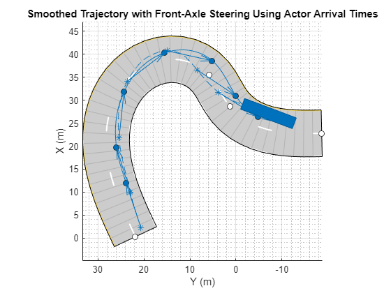
Create a trajectory for the vehicle, with reference to the front-axle for steering, using actor arrival times.

smoothTrajectory(egoVehicle,waypoints,TimeOfArrival=actorArrivalTimes,ReferenceSteerPosition="front-axle");

Plot the scenario, displaying the rear-axle trajecotry, and run the simulation. Observe the dashed line, which represents the rear-axle smoothed trajectory of the actor, created with reference to the front-axle steering using the actor arrival times.

plot(scenario,Waypoints="on",RoadCenters="on",ShowRearAxle="on")
title("Smoothed Trajectory with Front-Axle Steering Using Actor Arrival Times");
while advance(scenario)
    pause(0.1)
end

Input Arguments

ac — Actor

Actor object | Vehicle object

Actor belonging to a drivingScenario object, specified as an Actor or Vehicle object. To create these objects, use the actor and vehicle functions, respectively.

waypoints — Trajectory waypoints

real-valued N-by-2 matrix | real-valued N-by-3 matrix

Trajectory waypoints, in meters, specified as a real-valued N-by-2 or N-by-3 matrix. N is the number of waypoints.

• If waypoints is an N-by-2 matrix, then each matrix row represents the (x, y) coordinates of a waypoint. The z-coordinate of each waypoint is zero.

• If waypoints is an N-by-3 matrix, then each matrix row represents the (x, y, z) coordinates of a waypoint.

Each of the N – 1 segments between the waypoints defines a curve whose curvature varies linearly with length. If the first and last waypoint are identical, then the trajectory forms a loop.

Waypoints are in the world coordinate system.

Example: [1 0 0; 2 7 7; 3 8 8]

Data Types: single | double

speed — Speed of actor

30.0 (default) | real-valued scalar | N-element real-valued vector

Speed of the actor at each waypoint, in meters per second, specified as a real-valued scalar or N-element real-valued vector. N is the number of waypoints specified by waypoints.

• When speed is a scalar, the speed is constant throughout the actor motion.

• When speed is a vector, the vector values specify the speed at each waypoint. For forward motion, specify positive speed values. For reverse motion, specify negative speed values. To change motion directions, separate the positive and negative speeds by a waypoint with 0 speed.

Speeds are interpolated between waypoints. You can specify speed values as 0 at any waypoint but you cannot specify 0 speed at two consecutive waypoints.

If you do not specify speed, then by default, the actor travels at a constant speed of 30 m/s.

Example: [10 8 9] specifies speeds of 10 m/s, 8 m/s, and 9 m/s.

Example: [10 0 -10] specifies a speed of 10 m/s in forward motion, a pause for changing directions, and a speed of 10 m/s in reverse.

Data Types: single | double

waittime — Wait time of actor

0 (default) | N-element vector real-valued vector

Wait time of the actor at each waypoint, in seconds, specified as an N-element real-valued vector. N is the number of waypoints specified by waypoints.

When you specify a nonnegative wait time for the actor at a waypoint, the actor pauses at that waypoint for the specified number of seconds. When you specify a nonnegative wait time, you must set the corresponding speed value to 0. You can set the waitime to 0 at any waypoint, but you cannot set waittime at two consecutive waypoints to nonzero values.

Example: [0 0 5 0] pauses the actor for five seconds when it reaches the third waypoint.

Data Types: single | double

timeOfArrival — Time of actor arrival

N-element real-valued column vector

Since R2024b

Time of actor arrival, specified as an N-element real-valued column vector. N is the number of waypoints. Units are in seconds.

Example: [1 1.2 1.5] specifies actor arrival times of 1 s, 1.2 s, and 1.5 s.

Data Types: single | double | int8 | int16 | int32 | int64 | uint8 | uint16 | uint32 | uint64

Name-Value Arguments

Specify optional pairs of arguments as Name1=Value1,...,NameN=ValueN, where Name is the argument name and Value is the corresponding value. Name-value arguments must appear after other arguments, but the order of the pairs does not matter.

Example: smoothtrajectory(vehicle,waypoints,Course=course,ReferenceSteerPosition="front-axle") creates a smoothed trajectory for a vehicle, vehicle, from a set of waypoints, waypoints, using course angles at each waypoint, course, with reference to the front-axle for steering.

Before R2021a, use commas to separate each name and value, and enclose Name in quotes.

Course — Course angle

N-element real-valued column vector

Since R2024b

Course angle specifying the steering direction of the actor, specified as an N-element real-valued column vector, where N is the number of waypoints. Units are in degrees, and angles are positive in the counterclockwise direction.

If you do not specify Course, then the course angle at each waypoint is NaN, meaning that the course has no constraints.

Example: [0 90] specifies an actor at a 0-degree angle at the first waypoint and a 90-degree angle at the second waypoint.

Example: [0 NaN] specifies an actor at a 0-degree angle at the first waypoint. The actor has no constraints on its course at the second waypoint.

Data Types: single | double

Yaw — Yaw orientation angle of actor

N-element real-valued vector

Yaw orientation angle of the actor at each waypoint, in degrees, specified as the comma-separated pair consisting of 'Yaw' and an N-element real-valued vector. N is the number of waypoints specified by waypoints. Angles are positive in the counterclockwise direction.

If you do not specify yaw, then the yaw at each waypoint is NaN, meaning that the yaw has no constraints.

Example: [0 90] specifies an actor at a 0-degree angle at the first waypoint and a 90-degree angle at the second waypoint.

Example: [0 NaN] specifies an actor at a 0-degree angle at the first waypoint. The actor has no constraints on its yaw at the second waypoint.

Data Types: single | double

Jerk — Maximum longitudinal jerk of actor

0.6 (default) | real-valued scalar greater than or equal to 0.1

Maximum longitudinal jerk of the actor, in meters per second cubed, specified as the comma-separated pair consisting of 'Jerk' and a real-valued scalar greater than or equal to 0.1.

To limit jerk to a range that creates comfortable trajectories for human passengers, set 'Jerk' in the range from 0.3 to 0.9 [1].

Data Types: single | double

InitialHeading — Heading angle of actor at first waypoint

scalar

Since R2024b

Heading angle of the actor at the first waypoint, specified as a scalar. Units are in degrees.

If you do not specify InitialHeading, the function sets this value to align with the direction of the initial waypoint.

Note

To use the InitialHeading name-value argument, you must specify the ReferenceSteerPosition name-value argument as "front-axle".

Data Types: single | double

MotionDirection — Direction in which actor is moving

N-element numeric column vector | N-element string array

Since R2024b

Direction in which the actor is moving, specified as an N-element numeric column vector or an N-element string array. N is the number of waypoints.

• If you specify a numeric vector, use 1, -1, and 0 to represent forward, reverse, and stop, respectively.

• If you specify a string array, use "Forward", "Reverse", and "Stopped" to represent forward, reverse, and stop, respectively.

• By default, the MotionDirection value for each waypoint is "Forward".

• For an actor to perform reverse movement, you must stop the actor before reversing its direction. For example, to perform reverse movement in the form forward-stop-reverse, you must specify [1 0 -1].

Note

To use the MotionDirection name-value argument, you must specify the timeOfArrival input argument.

Example: [1 0 -1] specifies actor directions of forward, stop, and reverse at the first, second, and third waypoints, respectively.

Example: ["Forward","Stopped","Reverse"] specifies actor directions of forward, stop, and reverse at the first, second, and third waypoints, respectively.

Data Types: single | double | int8 | int16 | int32 | int64 | string

ReferenceSteerPosition — Reference steering position

"rear-axle" (default) | "front-axle"

Since R2024b

Reference steering position of the vehicle, specified as "rear-axle" or "front-axle". The function creates a trajectory for the actor ac with the steering location specified by this argument.

If you specify "front-axle", the input actor ac must be a Vehicle object. To create a Vehicle object, use the vehicle function. For more information, see the Create Smoothed Front-Axle Trajectory Using Actor Arrival Times example.

Example: "front-axle" creates a trajectory for a vehicle from a set of waypoints with reference to the front axle for steering.

Data Types: string

Tips

• If the smoothTrajectory function is unable to compute a smooth, jerk-limited trajectory given the input parameters, try making these adjustments to the scenario:

  • Extend the distances between waypoints to give the vehicle more time to accelerate to the specified speeds.

  • Lower the speeds at each waypoint. Try converting the speed values from meters per second to miles per hour to see if the speeds are realistic given the scenario. For example, the algorithm is unlikely to successfully compute a smooth trajectory for a sharp turn that is taken at a speed of 30 m/s (about 67 mph).

  • Increase the maximum jerk. Increasing the jerk maximum enables the algorithm to compute more possible trajectories, at the expense of reduced human passenger comfort.

• To get the position of the vehicle with reference to a specific vehicle body location, use the getReferencePosition function.

• If a driving scenario contains a front-axle trajectory for at least one vehicle, you can get the front-axle position from the FrontAxlePosition field of the ActorPoses structure returned by the record function.

• If a driving scenario contains a front-axle trajectory, to plot both the rear-axle and front-axle trajectories, specify the ShowRearAxle name-value argument of the plot function as "on".

Algorithms

The smoothTrajectory function creates a jerk-limited trajectory using a trapezoidal acceleration profile. This trajectory has smooth acceleration transitions between waypoints, resulting in a comfortable ride for human passengers. The function calculates a separate trapezoidal acceleration profile for each of the N - 1 segments between trajectory waypoints.

Consider a simple scenario in which a car travels a distance of 50 meters along a 100-meter road. The trajectory consists of one 50-meter segment in which the car must increase its speed from 5 m/s to 10 m/s by the end of the segment. The trajectory has an additional constraint in which the maximum longitudinal jerk must not exceed 0.5 m/s³.

scenario = drivingScenario;
car = vehicle(scenario);
road(scenario,[0 -25; 0 75]); % m
waypoints = [0 0; 0 50]; % m

speed = [5 10]; % m/s
jerk = 0.5; % m/s^3
smoothTrajectory(car,waypoints,speed,'Jerk',jerk)

Given the distance, speed, and jerk constraints of this waypoint segment, the smoothTrajectory function generates a three-phase trapezoidal acceleration profile:

1. Increase acceleration linearly. Hold jerk constant at a value no greater than jerk.

2. Hold acceleration constant. Decrease jerk to 0.

3. Decrease acceleration linearly. Hold jerk constant at a value no less than -jerk.

These plots visualize the distance, speed, acceleration, and jerk profile along this waypoint segment over time. The three phases of the acceleration profile form a trapezoidal shape.

When speed decreases between waypoints, the smoothTrajectory function generates the three-phase trapezoidal acceleration profile in reverse order. In the decreased speed case, the shape of the acceleration profile is the inverse of the one shown in the previous plot.

References

[1] Bae, Il, Jaeyoung Moon, and Jeongseok Seo. "Toward a Comfortable Driving Experience for a Self-Driving Shuttle Bus." Electronics 8, no. 9 (August 27, 2019): 943. https://doi.org/10.3390/electronics8090943.

Version History

Introduced in R2021a

R2024b: Additional input arguments

You can now specify the timeOfArrival input argument to create a trajectory based on actor arrival times at each waypoint.

The trajectory function now supports these additional name-value arguments:

• MotionDirection

• ReferenceSteerPosition

• Course

• InitialHeading

R2024b: Yaw name-value argument to be removed

The Yaw name-value argument will be removed in a future release. Use the Course name-value argument instead.