Compute Moving Variance of Noisy Square Wave Signal
Generate a noisy square wave signal using the Random Source block. Compute the moving variance of the signal using the Moving Variance block. Use the sliding window method with a hop size  of 5 and 1, and the exponential weighting method with a forgetting factor of 0.9 and 0.99. Compare the output of these two methods. For more details on these methods, see Sliding Window Method and Exponential Weighting Method.
Open and Run the Model
Open and run the MovVarModel.slx model.
The input is a noisy square wave signal. To control the power of the noise, multiply the noise generated by the Random Source block with a standard deviation value. Use a Pulse Generator (Simulink) block along with a Switch (Simulink) to vary the standard deviation between 0.08 and 0.12. Expected variance is the square of this value. The frame length of the input signal is 512 samples.
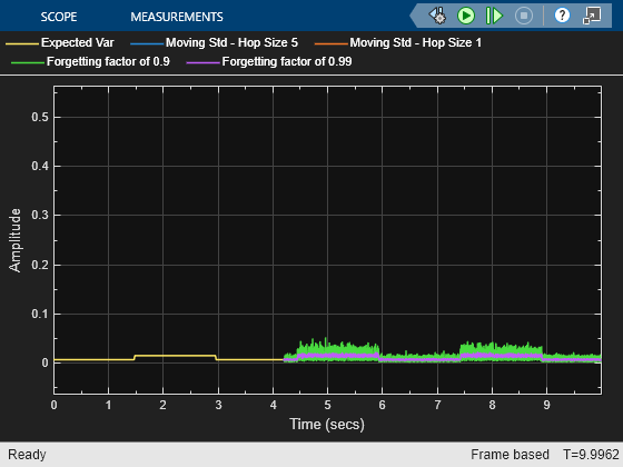
Compute the moving variance of the noisy square wave signal using four Moving Variance blocks. In the first two Moving Variance blocks that use the sliding window method, the window length is set to 100 and the overlap length is set to 95 and 99, respectively, resulting in a hop size of 5 and 1. In the last two Moving Variance blocks that use the exponential weighting method, the forgetting factor is set to 0.9 and 0.99, respectively. View and compare the outputs with the expected variance in the Time Scope.

Compare Moving Variance Outputs
In the sliding window Moving Variance blocks, when you select the Allow arbitrary frame length for fixed-size input signals parameter, the dimensions of the moving variance output change based on the hop size. If the input is  , then the output has an upper bound size of
  . For more details, see Moving Variance.
The last two blocks use the exponential weighting method. In the exponential weighting method, when the forgetting factor is low, past data has a lower impact on the current output. If the signal changes rapidly as in this example, use a low forgetting factor. This makes the transient sharper even though the output contains more noise. You can see this behavior in the Time Scope when you compare the moving variance outputs for the forgetting factors 0.9 and 0.99.

See Also
Random Source | Pulse Generator (Simulink) | Constant (Simulink) | Switch (Simulink) | Moving Variance | Time Scope