Solve Feasibility Problem Using surrogateopt, Problem-Based

Some problems require you to find a point that satisfies all constraints, with no objective function to minimize. For example, suppose that you have the following constraints:

$$\begin{array}{l}(y+x^2{)}^2+0.1y^2\le 1\\ y\le \exp (-x)-3\\ y\le x-4.\end{array}$$

Do any points $$(x,y)$$ satisfy the constraints? To answer this question, you need to evaluate the expressions at a variety of points. The surrogateopt solver does not require you to provide initial points, and it searches a wide set of points. So, surrogateopt works well for feasibility problems.

To visualize the constraints, see Visualize Constraints. For a solver-based approach to this problem, see Solve Feasibility Problem.

Note: This example uses two helper functions, outfun and evaluateExpr. The code for each function is provided at the end of this example. Make sure the code for each function is included at the end of your script or in a file on the path.

Set Up Feasibility Problem

For the problem-based approach, create optimization variables x and y, and create expressions for the listed constraints. To use the surrogateopt solver, you must set finite bounds for all variables. Set lower bounds of –10 and upper bounds of 10.

x = optimvar("x","LowerBound",-10,"UpperBound",10);
y = optimvar("y","LowerBound",-10,"UpperBound",10);
cons1 = (y + x^2)^2 + 0.1*y^2 <= 1;
cons2 = y <= exp(-x) - 3;
cons3 = y <= x - 4;

Create an optimization problem and include the constraints in the problem.

prob = optimproblem("Constraints",[cons1 cons2 cons3]);

The problem has no objective function. Internally, the solver sets the objective function value to 0 for every point.

Solve Problem

Solve the problem using surrogateopt.

rng(1) % For reproducibility
[sol,fval] = solve(prob,"Solver","surrogateopt")

Solving problem using surrogateopt.

surrogateopt stopped because it exceeded the function evaluation limit set by 
'options.MaxFunctionEvaluations'.

sol = struct with fields:
    x: 1.7087
    y: -2.8453

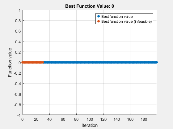
fval = 0

The first several evaluated points are infeasible, as indicated by the color red in the plot. After about 60 evaluations, the solver finds a feasible point, plotted in blue.

Check the feasibility at the returned solution.

infeasibility(cons1,sol)

ans = 0

infeasibility(cons2,sol)

ans = 0

infeasibility(cons3,sol)

ans = 0

All infeasibilities are zero, indicating that the point sol is feasible.

Stop Solver at First Feasible Point

To reach a solution faster, create an output function (see Output Function) that stops the solver whenever it reaches a feasible point. The outfun helper function at the end of this example stops the solver when it reaches a point with no constraint violation.

Solve the problem using the outfun output function.

opts = optimoptions("surrogateopt","OutputFcn",@outfun);
rng(1) % For reproducibility
[sol,fval] = solve(prob,"Solver","surrogateopt","Options",opts)

Solving problem using surrogateopt.

Optimization stopped by a plot function or output function.

sol = struct with fields:
    x: 1.7087
    y: -2.8453

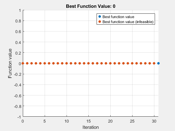
fval = 0

This time, the solver stops earlier than before.

Visualize Constraints

To visualize the constraints, plot the points where each constraint function is zero by using fimplicit. The fimplicit function passes numeric values to its functions, whereas the evaluate function requires a structure. To tie these functions together, use the evaluateExpr helper function, which appears at the end of this example. This function simply puts passed values into a structure with the appropriate names.

Avoid a warning that occurs because the evaluateExpr function does not work on vectorized inputs. Plot the returned solution point as a green circle.

s = warning('off','MATLAB:fplot:NotVectorized');
figure
cc1 = (y + x^2)^2 + 0.1*y^2 - 1;
fimplicit(@(a,b)evaluateExpr(cc1,a,b),[-2 2 -4 2],'r')
hold on
cc2 = y - exp(-x) + 3;
fimplicit(@(a,b)evaluateExpr(cc2,a,b),[-2 2 -4 2],'k')
cc3 = y - x + 4;
fimplicit(@(x,y)evaluateExpr(cc3,x,y),[-2 2 -4 2],'b')
plot(sol.x,sol.y,'og')
hold off

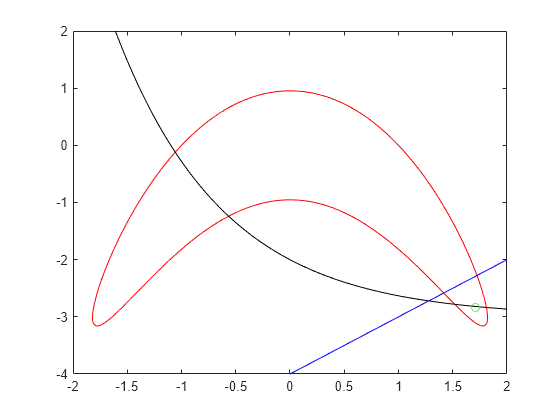
warning(s);

The feasible region is inside the red outline and below the black and blue lines. The feasible region is at the lower right of the red outline.

Helper Functions

This code creates the outfun helper function.

function stop = outfun(~,optimValues,state)
stop = false;
switch state
    case 'iter'
        if optimValues.currentConstrviolation <= 0
            stop = true;
        end
end
end

This code creates the evaluateExpr helper function.

function p = evaluateExpr(expr,x,y)
pt.x = x;
pt.y = y;
p = evaluate(expr,pt);
end