Analyze Performance of Code Generated for Deep Learning Networks
This example shows how to analyze the performance of CUDA® code generated for deep learning networks by using the gpuPerformanceAnalyzer function.
The gpuPerformanceAnalyzer function generates code and collects metrics on CPU and GPU activities in the generated code. The function generates a report that contains a chronological timeline plot that you can use to visualize and identify performance bottlenecks in the generated CUDA code. Additionally, the report contains a dashboard that you can use to analyze the deep learning network's performance.
This example generates the performance analysis report for a function that uses a deep learning variational autoencoder (VAE) to generate digit images. For more information, see Generate Digit Images on NVIDIA GPU Using Variational Autoencoder.
Third-Party Prerequisites
CUDA-enabled NVIDIA® GPU.
NVIDIA CUDA toolkit and driver. For information on the supported versions of the compilers and libraries, see Third-Party Hardware.
Environment variables for the compilers and libraries. For setting up the environment variables, see Setting Up the Prerequisite Products.
Verify GPU Environment
To verify that the compilers and libraries for this example are set up correctly, use the coder.checkGpuInstall function.
envCfg = coder.gpuEnvConfig("host");
envCfg.DeepLibTarget = "cudnn";
envCfg.DeepCodegen = 1;
envCfg.Quiet = 1;
coder.checkGpuInstall(envCfg);
When the Quiet property of the coder.gpuEnvConfig object is set to true, the coder.checkGpuInstall function returns only warning or error messages.
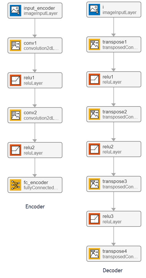
Analyze the Pretrained Variational Autoencoder Network
Autoencoders have two parts: the encoder and the decoder. The encoder takes an image input and outputs a compressed representation. The decoder takes this compressed representation, decodes it, and recreates the original image.
VAEs differ from regular autoencoders in that they do not use the encoding-decoding process to reconstruct an input. Instead, they impose a probability distribution on the latent space, and learn the distribution so that the distribution of outputs from the decoder matches that of the observed data. Then, they sample from this distribution to generate new data.
This example uses the decoder network trained in the Train Variational Autoencoder (VAE) to Generate Images (Deep Learning Toolbox) example. The encoder outputs a compressed representation that is a vector of size latent_dim. In this example, the value of latent_dim is equal to 20.
Examine the Entry-Point Function
The generateVAE entry-point function loads the dlnetwork object from the trainedDecoderVAENet MAT file into a persistent variable and reuses the persistent object during subsequent prediction calls. It initializes a dlarray object that contains 25 randomly generated encodings, passes them through the decoder network, and extracts the numeric data of the generated image from the deep learning array object.
type("generateVAE.m")function generatedImage = generateVAE(decoderNetFileName,latentDim,Environment) %#codegen
% Copyright 2020-2021 The MathWorks, Inc.
persistent decoderNet;
if isempty(decoderNet)
decoderNet = coder.loadDeepLearningNetwork(decoderNetFileName);
end
% Generate random noise
randomNoise = dlarray(randn(1,1,latentDim,25,'single'),'SSCB');
if coder.target('MATLAB') && strcmp(Environment,'gpu')
randomNoise = gpuArray(randomNoise);
end
% Generate new image from noise
generatedImage = sigmoid(predict(decoderNet,randomNoise));
% Extract numeric data from dlarray
generatedImage = extractdata(generatedImage);
end
Generate GPU Performance Analyzer Report
To analyze the performance of the generated code, use the gpuPerformanceAnalyzer function. First, create a code configuration object with a MEX build type by using the mex input argument.
cfg = coder.gpuConfig("mex");Use the coder.DeepLearningConfig function to create a cuDNN deep learning configuration object and assign it to the DeepLearningConfig property of the GPU code configuration object.
cfg.TargetLang = "C++";
cfg.GpuConfig.EnableMemoryManager = true;
cfg.DeepLearningConfig = coder.DeepLearningConfig("cudnn");
Run gpuPerformanceAnalyzer with the default iteration count of 2. The GPU Performance Analyzer collects performance data for both iterations and opens automatically.
latentDim = 20;
Env = "gpu";
matfile = "trainedDecoderVAENet.mat";
inputs  = {coder.Constant(matfile), coder.Constant(latentDim), coder.Constant(Env)};
designFileName = "generateVAE";

gpuPerformanceAnalyzer(designFileName, inputs, ...
    "Config", cfg, "NumIterations", 2);
### Starting GPU code generation
Code generation successful: View report

### GPU code generation finished
### Starting application profiling
### Application profiling finished
### Starting profiling data processing
### Profiling data processing finished
### Showing profiling data
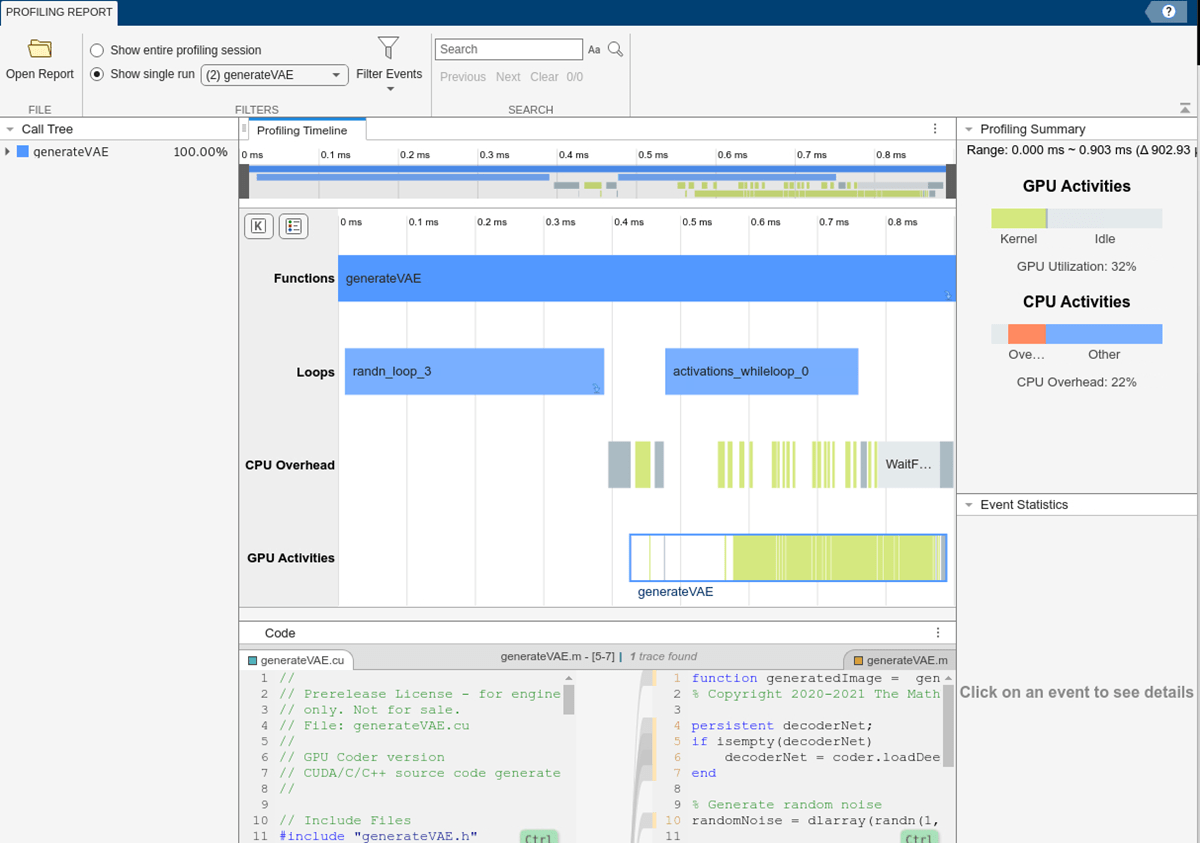
For this example, the values in the app depend on your hardware. The profiling in this example was performed using MATLAB® R2025a on a machine with a 13th gen Intel® Core™ i9-13900K CPU and an NVIDIA Titan V GPU.
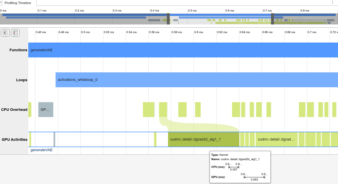
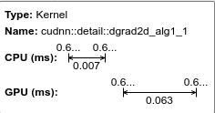
The Profiling Timeline shows the trace of the events on the CPU and GPU. In this example, the timeline shows that most of the execution time is due to events in the GPU Activities row. Additionally, the Profiling Summary shows that the GPU utilization is 85%. Use the mouse wheel or a touchpad to zoom in on the events in the Loops row. In the Loops row, the application contains a loop named activations_whileloop_0 for activations for the network.
Analyze Network Performance in the Deep Learning Dashboard
Next, analyze the runtime statistics for the network using the Deep Learning Dashboard.
Open the Deep Learning Dashboard
In the toolstrip, click Show Predict Functions to see the deep learning inference functions in the Profiling Timeline. The Show Predict Functions button is enabled because the entry-point function uses a deep learning network.
The Performance Analyzer marks deep learning events with a network icon. In this run, there is one predict function, dlnetwork_predict.
Select dlnetwork_predict. In the toolstrip, click Open Deep Learning Dashboard. Alternatively, in the toolbar that appears above dlnetwork_predict, click the Network button. The dashboard shows the runtime statistics from dlnetwork_predict.
Examine Execution Overview
The Execution Overview section shows the time the network took to execute and estimates the network efficiency as a percent.
In this example, the Execution Overview shows the network took 0.37ms out of the 0.56ms needed to run the entire entry-point function. The Network Efficiency estimates the efficiency of the network as a percent based on the runtime statistics. In this example, the network has an efficiency over 99%, which indicates that the generated code for the network is well-optimized and uses the GPU efficiently.
Analyze Network Runtime
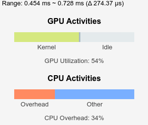
Use the Runtime Breakdown section to view the CPU and GPU activities during the network execution. This section displays the cumulative CPU and GPU activities side-by-side over the network execution time. In the Runtime Breakdown, in the GPU row, point to the green rectangle. A tooltip shows the GPU spent approximately 92% of the network execution time on computation or kernel execution.

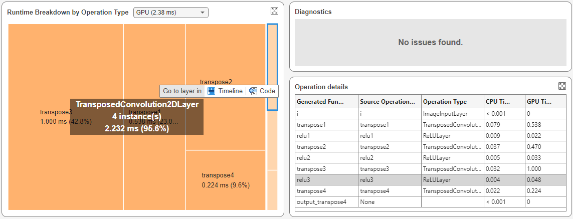
Analyze Runtime by Operation Type
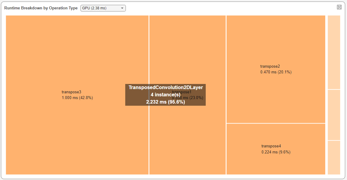
To identify the layer types that take the longest to execute, use the Runtime Breakdown by Operation Type pane. You view either the CPU or GPU execution times. In the Runtime Breakdown by Operation Type section, in the Select a Device list, select GPU.
The tree map groups the layers based on their type and displays layers that take longer to execute with more area. In this example, the tree map shows transposed 2-D convolution layers as the layer type that takes the longest to execute on the GPU, taking more than 95% of the execution time.
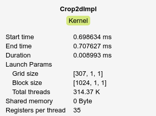
Layers that execute for very short periods do not have labels in the Runtime Breakdown by Operation Type pane. To determine the types of these layers, select them in the Runtime Breakdown by Operation Type pane. In this example, after selecting one of these layers, the Operation Details table shows that the layer is the Rectified Linear Unit (ReLU) layer named relu3.