Combine Landsat 9 Multispectral Images Using Image Mosaicing
This example shows how to stitch multiple Landsat 9 multispectral images into a mosaic image and analyze the mosaic image.
Landsat 9 Level-2 Surface Reflectance products provide atmospherically corrected multispectral data. This data is similar to data from Landsat 8. You can use Landsat 9 Level-2 Surface Reflectance data for consistent and high-quality monitoring of the Earth surface, for applications such as land cover mapping, vegetation analysis, and environmental change detection. Landsat 9 Level-2 Surface Reflectance products contain up to 11 spectral bands. This example uses these eight bands to cover key wavelengths for analyzing land surfaces and vegetation.
Coastal Aerosol
Blue
Green
Red
Near-Infrared (NIR)
Shortwave Infrared 1 (SWIR 1)
Shortwave Infrared 2 (SWIR 2)
Thermal Infrared 1
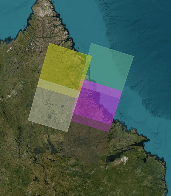
This example uses four Landsat 9 multispectral tile images that cover the eastern part of Quebec, Canada, near the western shore of the Labrador Sea. In this example, you combine the four Landsat 9 multispectral images into a single mosaic multispectral image and compute spectral indices for the mosaic image.
This example requires the Hyperspectral Imaging Library for Image Processing Toolbox™. You can install the Hyperspectral Imaging Library for Image Processing Toolbox from Add-On Explorer. For more information about installing add-ons, see Get and Manage Add-Ons. The Hyperspectral Imaging Library for Image Processing Toolbox requires desktop MATLAB®, as MATLAB® Online™ and MATLAB® Mobile™ do not support the library.
Download Data
This example uses four Landsat 9 multispectral tile images that cover a contiguous area of the eastern part of Quebec, Canada, near the western shore of the Labrador Sea. The tiles are approximately temporally consistent, but not radiometrically or atmospherically corrected. You can apply preprocessing such as cloud masking or surface normalization, if required for your application.
Download the data and unzip the file by using the downloadLandsat9Dataset helper function. The helper function is attached to this example as a supporting file.
zipfile = "landsat9_mosaic.zip";
landsat9Data_url = "https://ssd.mathworks.com/supportfiles/image/data/" + zipfile;
downloadLandsat9Dataset(landsat9Data_url,pwd)
Downloading the Landsat 9 dataset.
This can take several minutes to download...
Done.
Load Data
Load each of the four Landsat 9 tile images from the MTL files into the workspace as a multicube object with geospatial information by using the geomulticube function. Store all four multispectral images as a cell array of multicube objects.
imageFolders = {fullfile("landsat9_mosaic","LC09_L2SP_009020_20250303_20250305_02_T1","LC09_L2SP_009020_20250303_20250305_02_T1_MTL"), ...
fullfile("landsat9_mosaic","LC09_L2SP_009021_20250303_20250305_02_T1","LC09_L2SP_009021_20250303_20250305_02_T1_MTL"), ...
fullfile("landsat9_mosaic","LC09_L2SP_011020_20250301_20250302_02_T1","LC09_L2SP_011020_20250301_20250302_02_T1_MTL"), ...
fullfile("landsat9_mosaic","LC09_L2SP_011021_20250301_20250302_02_T2","LC09_L2SP_011021_20250301_20250302_02_T2_MTL")};
mcubeList = cell(1,length(imageFolders));
for i = 1:length(imageFolders)
txtFile = strcat(imageFolders{i},".txt");
if ~isfile(txtFile)
error("No .txt file found in %s",txtFile)
end
mcubeList{i} = geomulticube(txtFile);
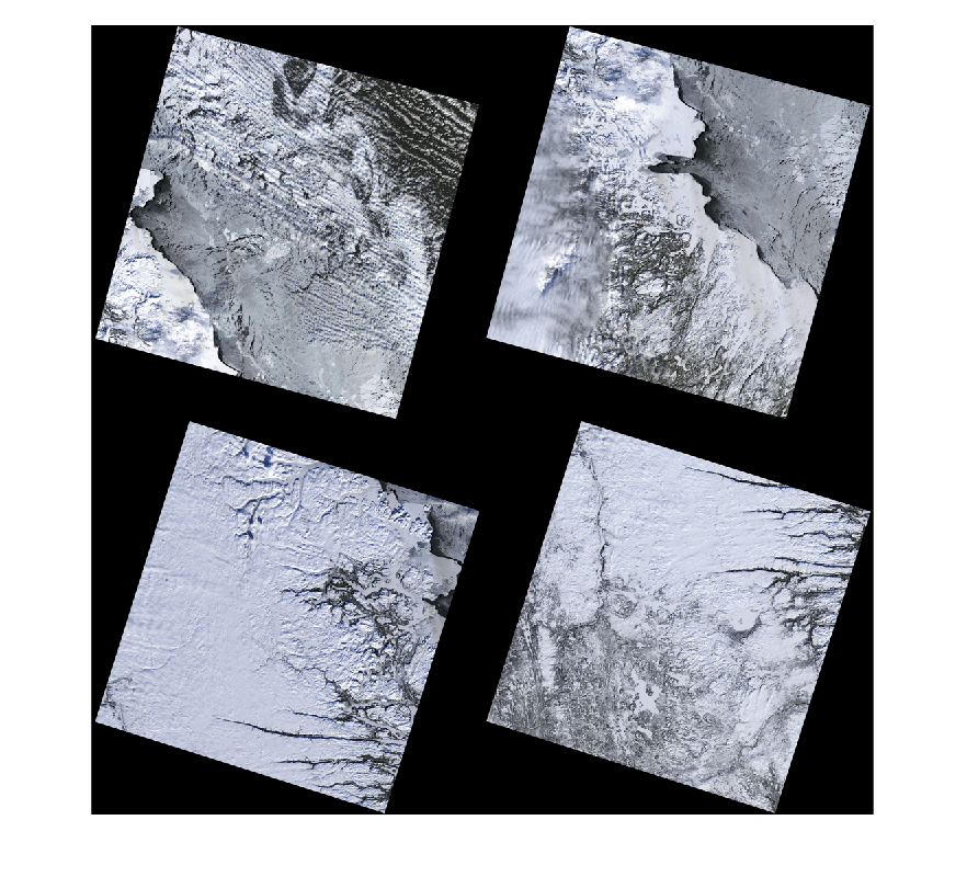
endVisualize the RGB images of the tiles.
rgbImages = cell(1,numel(mcubeList));
for i = 1:numel(mcubeList)
    rgbImages{i} = colorize(mcubeList{i},[4 3 1]);
end
figure
montage(rgbImages,Size=[2 2])
Compute Canvas Size for Mosaic
Compute the spatial extent required to contain all four tiles by using the helperComputeCanvasSize helper function. The helper function is attached to this example as a supporting file. The helperComputeCanvasSize function computes the minimum and maximum X- and Y-world coordinates for a space that contains all four tiles and returns a common raster reference for all bands. It also computes and returns the canvas size, in pixels, by dividing the spatial extent in world coordinate units by the pixel size.
[canvasGeoRef,canvasSize] = helperComputeCanvasSize(mcubeList);
The helperComputeCanvasSize function is specific to Landsat 9 multispectral images. You might need to modify the function to use it with multispectral images from different sensors.
Determine Tile Image Locations
Each multispectral tile image has spatial reference information that determines where it lies in the larger canvas. Use this information to calculate row and column indices for each image.
numImages = numel(mcubeList);
numBands = size(canvasSize,1);
imageLocation = cell(numBands,numImages);

for b = 1:numBands
    for i = 1:numImages
        ref = mcubeList{i}.Metadata.RasterReference(b);
        canvasRef = canvasGeoRef(b);
        [xi,yi] = worldToDiscrete(canvasRef,ref.XWorldLimits,ref.YWorldLimits);
        rowStart = min(xi);
        rowEnd = max(xi);
        colStart = min(yi);
        colEnd = max(yi);
        imageLocation{b,i} = [rowStart rowEnd colStart colEnd];
    end
end
Perform Image Mosaicing
For each spectral band, extract the band image from each tile, and ensure all values are nonnegative by scaling the band image to the range [0, 1]. Place the band image from each tile onto the canvas using the computed image location.
Use a sign-based weights to avoid overwriting existing data. In overlapping regions, write new data only to pixels with a value of 0.
When a canvas pixel is blank, it has a value of zero. The sign-based weight
Wassigns a weight of0to the canvas pixel and a weight of1to the band image pixel being written to that position of the canvas in that location.When a canvas pixel has been filled, it has a positive value due to the band image scaling. The sign-based weight
Wassigns a weight of1to the canvas pixel and a weight of0to the new band image pixel being written to the canvas in that location.
Save each mosaic band as a GeoTIFF file using the WGS 84 / UTM zone 20N coordinate system, which is applicable to the location of Quebec, Canada.
for b = 1:numBands
    filename = sprintf("mosaicImage_%d.tif",b);
    if exist(filename,"file")
        delete(filename)
    end
end

for b = 1:numBands
    fileOut = sprintf("mosaicImage_%d.tif",b);
    canvas = zeros(canvasSize(b,1:2));
    for i = 1:numImages
        loc = imageLocation{b,i};
        mcubeBand = selectBands(mcubeList{i},BandNumber=b);
        mcubeBand = gather(mcubeBand);
        mcubeBand = im2double(mcubeBand);
        W = sign(canvas(loc(1):loc(2),loc(3):loc(4)));
        canvas(loc(1):loc(2),loc(3):loc(4)) = (canvas(loc(1):loc(2),loc(3):loc(4)).*W + mcubeBand.*(1-W));
    end
    geotiffwrite(fileOut,canvas,canvasGeoRef(b),CoordRefSysCode=32620)
end
Update Metadata for the Stitched Mosaic
Landsat metadata includes geospatial attributes, band filenames, and corner coordinates. Update the metadata of the mosaic multispectral image by using the helperUpdateMetadata helper function. The helper function is attached to this example as a supporting file.
MTLFileName = "LC09_L2SP_new_MTL.txt";
if exist(MTLFileName,"file")
    delete(MTLFileName)
end
inputFile = fullfile("landsat9_mosaic","LC09_L2SP_009020_20250303_20250305_02_T1","LC09_L2SP_009020_20250303_20250305_02_T1_MTL.txt");
helperUpdateMetadata(inputFile,MTLFileName,canvasGeoRef(1));
The helperUpdateMetadata function is specific to Landsat 9 multispectral images. You might need to modify the function to use it with multispectral images from different sensors.
Use the updated metadata file to read the mosaic multispectral image into the workspace as a multicube object.
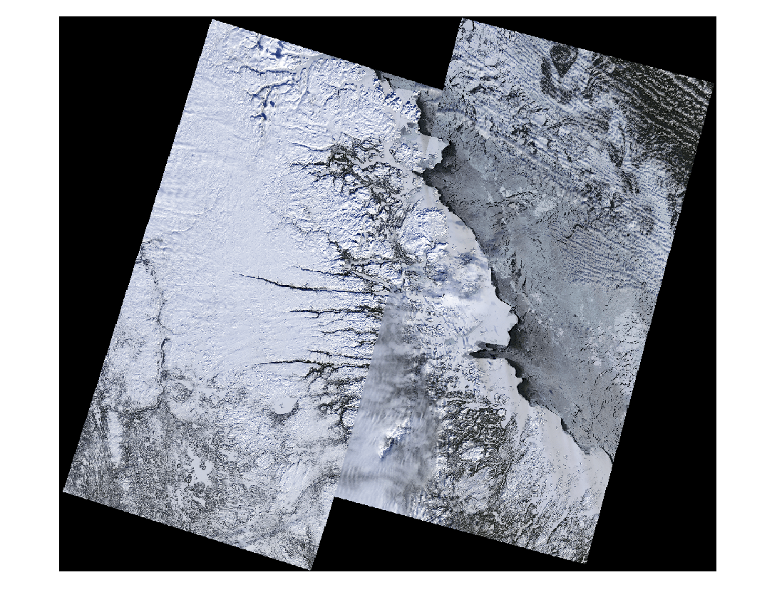
mcubeStitch = immulticube("LC09_L2SP_new_MTL.txt");Visualize the RGB image of the mosaic multispectral image.
colorImg = colorize(mcubeStitch,[4 3 1]);
dispColorImg = imresize(colorImg,0.35);
figure
imshow(dispColorImg)
Compute Spectral Indices
Vegetation indices help quantify vegetation vigor and coverage. Compute the Green Vegetation Index (GVI) by using the spectralIndices function. Threshold the GVI map to detect vegetation. You can tune the threshold for specific land cover types or environmental conditions.
indicesGVI = spectralIndices(mcubeStitch,"GVI");
indexMapGVI = indicesGVI.IndexImage;
threshGVI = 0;
maskGVI = indexMapGVI > threshGVI;
Compute the Normalized Difference Snow Index (NDSI) spectral index by using customSpectralIndex function. The NDSI index requires green and SWIR wavelengths for computation. Threshold the NDSI map to detect snow.
func = @(b1,b2) (b1-b2)./(b1+b2);
indexMapNDSI = customSpectralIndex(mcubeStitch,[556 1610],func);
threshNDSI = 0.55;
maskNDSI = indexMapNDSI > threshNDSI;
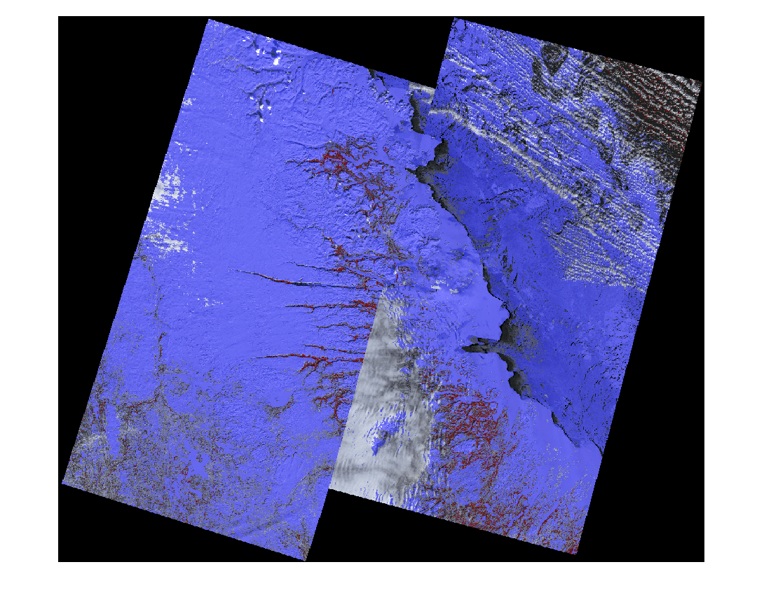
Overlay the thresholded spectral indices result on an RGB image of the mosaic multispectral image. Color the GVI overlay red and the NDSI overlay blue.
overlayImg = labeloverlay(colorImg,maskGVI,Colormap=[1 0 0],Transparency=0.5);
overlayImg = labeloverlay(overlayImg,maskNDSI,Colormap=[0 0 1],Transparency=0.5);
dispOverlayImg = imresize(overlayImg,0.35);
figure
imshow(dispOverlayImg)
You can perform image mosaicing to stitch multiple Landsat scenes into a seamless mosaic, update metadata, and analyze the results for various applications such as land cover classification, vegetation health monitoring, urban growth studies, regional planning, and water and soil assessment. You can also apply deep learning models on the mosaic image to perform segmentation and change detection.