Explore 3-D Labeled Volumetric Data with Volume Viewer

This example shows how to explore 3-D labeled volumetric data using the Volume Viewer app. Using the app, you can view the labels by themselves or as an overlay on the intensity volume. To illustrate, the example loads an intensity volume that shows the human brain with labeled areas that show the location and type of tumors found in the brain.

Load Labeled Volume and Intensity Volume

Load the MRI intensity data of a human brain and the labeled volume from MAT files into the workspace. The MRI data is a modified subset of the BraTS data set [1]. This operation creates two variables in the workspace: vol and label.

datadir = fullfile(toolboxdir("images"),"imdata","BrainMRILabeled");
load(fullfile(datadir,"images","vol_001.mat"))
load(fullfile(datadir,"labels","label_001.mat"))
whos

  Name           Size                    Bytes  Class     Attributes

  datadir        1x1                       422  string              
  label        240x240x155             8928000  uint8               
  vol          240x240x155            17856000  uint16              

Open the Volume Viewer app. From the MATLAB® Toolstrip, open the Apps tab and, under Image Processing and Computer Vision, click Volume Viewer. You can also open the app by using the volumeViewer command.

volumeViewer

Load the labeled volume into the Volume Viewer app. In the Viewer tab of the app toolstrip, select Import and choose an option under Labels. You can load labels from a file, or as a variable from the workspace. Loading from a file is useful if the label volume has nonuniform voxel spacing that is specified in the file metadata. If you have volumetric data in a DICOM format that uses multiple files to represent a volume, you can specify the DICOM folder name. For this example, under Data, choose From Workspace. The app assumes uniform voxel spacing of 1-by-1-by-1 mm.

Select the workspace variable associated with the labeled volume data label in the Import Labels dialog box and click OK.

View Labeled Volume in Volume Viewer

By default, Volume Viewer displays the data as three 2-D slice planes and a 3-D volume in a four-pane view. You can change the layout to focus on one pane by selecting Layout in the app toolstrip and, under Focus, the pane you want to focus on.

To explore the volume, zoom in and out on any of the display panes using the mouse wheel, or by selecting the zoom icon in the top-right corner of the pane and clicking the image. Navigate between 2-D slices by using the scroll bar in each of the 2-D slice panes. Labels in the bottom-left corner of each slice pane indicate the current slice number and the total number of slices in that dimension. The bottom of the app window displays information about the pixel beneath the mouse pointer, including its coordinates and intensity.

In the 3-D Volume pane, you can drag the volume to rotate it about its center. The orientation axes in the bottom-left corner indicate the spatial orientation of the volume. The scale bar in the bottom-right corner provides an indication of the volume size. You can toggle the visibility of the orientation axes and scale bar by selecting Display Markers in the app toolstrip and selecting or clearing options.

Optionally, you can adjust the visibility and opacity of all labels by selecting View Labels or by dragging the Label Opacity slider, respectively, in the app toolstrip. You can also toggle the visibility or change the color of individual labels from the Labels pane of the app window. To change the color for a label, click the corresponding rectangle in the Color column of the table and select a new color in the picker window. To show or hide a label, click the corresponding eye icon in the Show/Hide column of the table.

View Labels as Overlay on Intensity Volume

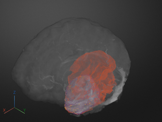
Viewing the labels overlaid on the intensity volume can provide context for the data. For this example, use the overlay to locate the tumor within the full brain.

With the labeled volume already in the Volume Viewer, load the intensity volume into the app. In the Viewer tab of the app toolstrip, select Import and, under Data, choose From Workspace.

Select the workspace variable associated with the intensity volume vol in the Import Volume dialog box and click OK.

The Volume Viewer displays the labeled volume over the intensity volume data. You can adjust the transparency of the labels over the intensity volume by using the Label Opacity slider in the app toolstrip. You can also toggle the visibility of all labels or the volume by selecting View Labels and View Volume, respectively.

You can refine the intensity volume display using options in the Rendering Editor.

• Choose the rendering technique from these options: Gradient Opacity (default), Volume Rendering, Cinematic Rendering, Minimum Intensity Projection, Maximum Intensity Projection, Isosurface, and Slice Planes.

• Modify the transparency alphamap by specifying a preset alphamap, such as CT_Bone, or by customizing the alphamap using the intensity-opacity curve.

• Modify the colormap by specifying a built-in colormap like jet or CT_Bone or by importing a colormap from the workspace. You can refine the colormap using the interactive color bar scale.

For details about each rendering technique and the alphamap and colormap options, see Explore 3-D Volumetric Data with Volume Viewer.

Save Volume Viewer Rendering and Camera Configuration Settings

After configuring Volume Viewer for the best view of your data, you can save your rendering settings and camera configuration to the workspace. You can apply the saved settings to recreate the view you achieved in Volume Viewer by using them to set properties of the objects created by the viewer3d and volshow functions.

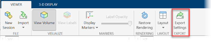
To save rendering and camera configuration settings, in the Viewer tab of the app toolstrip, click Export Settings.

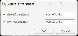
Volume Viewer creates separate structures for the settings of objects created by viewer3d and volshow. In the Export To Workspace dialog box, you can choose which structures to create, and either specify their names or accept the default names of sceneConfig and objectConfig, respectively. When you are ready to export, click OK.

Apply Rendering Settings Outside App

Programmatically display the volume, applying the rendering and camera settings from the app. The new display has the same colormap, alphamap, rendering style, background color, and camera position as the 3-D Volume pane had when you exported the settings. Note that this example loads and applies rendering settings attached to the example as a supporting file.

load("labelVolSettings.mat")

% Create volume display

viewer = viewer3d;

Volume = volshow(vol,Parent=viewer, ...
    DisplayRangeMode="data-range", ...
    OverlayData=label);

% Set the volume rendering preset values for main data and overlay data

fields = fieldnames(objectConfig);
for i = 1:numel(fields)
    Volume.(fields{i}) = objectConfig.(fields{i});

end

% Set the camera and background settings

fields = fieldnames(sceneConfig);
for i = 1:numel(fields)

    viewer.(fields{i}) = sceneConfig.(fields{i});
end

References

[1] Medical Segmentation Decathlon. "Brain Tumours." Tasks. Accessed May 10, 2018. http://medicaldecathlon.com/.

The BraTS data set is provided by Medical Segmentation Decathlon under the CC-BY-SA 4.0 license. All warranties and representations are disclaimed. See the license for details. MathWorks® has modified the subset of data used in this example. This example uses the MRI data of one scan from the original data set, saved to a MAT file.