Graph Coloring with Grover's Algorithm

This example shows how to use Grover's algorithm on a quantum computer to solve graph coloring problems. Grover's algorithm, also called the quantum search algorithm, is a fast method to perform unstructured searches. This example applies the algorithm to a problem where a bit string of a given length is classified as valid or invalid, and the goal is to retrieve one of the valid bit strings. The algorithm uses a state oracle to determine whether a bit string is valid. Although this application of Grover's algorithm is not the most efficient method to solve the graph coloring problem in practice, it illustrates how a quantum algorithm can be applied to a well-known problem.

Create State Oracle for Graph Coloring Problem

Create a graph with four nodes and four edges connecting them.

g = graph([2 2 3 3],[1 4 1 4]);
plot(g)

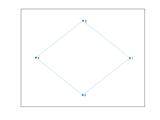
Because the graph has only four nodes and four edges, there are a limited number of ways to color the nodes in the graph. If each node can be one of two different colors, then there are $2^4=16$ ways to color the graph nodes.

A solution of the graph coloring problem is a color assignment such that adjacent nodes are not the same color. Therefore, the quantum state oracle must check that for each edge in a given graph, the nodes it connects have different colors. The oracle accomplishes this check by accepting a bit string of length 4 (represented by 4 qubits), each of which represents the color of one node, and determining whether the colors produce a valid graph coloring.

Create Oracle

As a first step to creating the oracle, create a helper circuit called xorGate. This circuit reads qubits 1 and 2, and flips qubit 3 from $\left|0\right.anglebracketright$ to $\left|1\right.anglebracketright$ if qubits 1 and 2 have different values.

xorInnerGates = [cxGate(1,3);
                 cxGate(2,3)];
xorGate = quantumCircuit(xorInnerGates,Name="XOR");

Next, loop through all edges in the graph and write the value of xorGate applied to the startNode and endNode qubits into a new helper qubit representing the edge. This increases the number of qubits from 4 to 8 because there are four edges. The first four qubits represent the bit string to evaluate, while the other qubits begin in state $\left|0\right.anglebracketright$ before xorGate is applied.

[startNodes,endNodes] = findedge(g);
N = numnodes(g);
E = numedges(g);
gates = [];
for k = 1:E
  gates = [gates; 
           compositeGate(xorGate,[startNodes(k),endNodes(k),N+k])];
end

Next, the oracle must verify that the helper qubits representing the edges are in state $\left|1\right.anglebracketright$, since xorGate returns $\left|1\right.anglebracketright$ when the two nodes connected by the edge have different states. This verification requires the addition of a ninth qubit that has a state of $\left|1\right.anglebracketright$ when the coloring is valid, and $\left|0\right.anglebracketright$ otherwise. Use the mcxGate function to determine the value of this final qubit, and create a circuit for the oracle.

lastQubit = N+E+1;
gates = [gates; 
         mcxGate(N+(1:E),lastQubit,[])];
oracle = quantumCircuit(gates,lastQubit);
oracle.Name = "Oracle"

oracle = 
  quantumCircuit with properties:

    NumQubits: 9
        Gates: [5×1 quantum.gate.CompositeGate]
         Name: "Oracle"

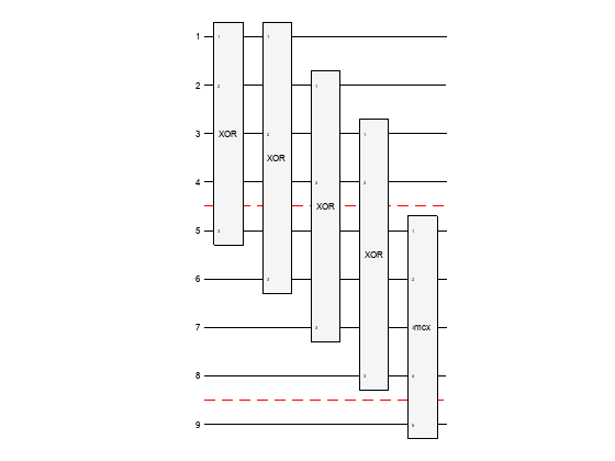
Plot the circuit representing the oracle to view all of the qubits and gates. Use the QubitBlocks option to draw red lines between the different groups of qubits: the first four qubits at the top of the circuit diagram represent the node colors being checked, the next four qubits are the helper qubits to check the nodes connected by each edge, and the final qubit at the bottom determines whether the graph coloring is valid.

plot(oracle,QubitBlocks=[4 4 1])

Check Initial Oracle Behavior

Construct two input configurations, one valid (1001) and one invalid (1111), and apply the oracle circuit to each of them to check its behavior. The input configuration is encoded in the left-most four characters of each bit string, and the value of interest is the last qubit (the right-most character) in the output bit string.

Start with the invalid coloring 1111, where all nodes are the same color.

invalidColors = "111100000";
inputState1 = quantum.gate.QuantumState(invalidColors);
formula(inputState1)

ans = 
"1 * |111100000>"

Apply the oracle to see the output state.

outputState1 = simulate(oracle,inputState1);
formula(outputState1)

ans = 
"1 * |111100000>"

The last qubit of the simulated state is 0, so the oracle correctly determines that not all of the nodes can be the same color. Next, check the coloring 1001.

validColors = "100100000";
inputState2 = quantum.gate.QuantumState(validColors);
formula(inputState2)

ans = 
"1 * |100100000>"

Again, apply the oracle to see the output state.

outputState2 = simulate(oracle, inputState2); 
formula(outputState2)

ans = 
"1 * |100111111>"

In this case, the last qubit is 1, so 1001 is a valid graph coloring, where each edge connects nodes of different colors. This check confirms that the behavior of the oracle is correct for these two cases.

Refine Oracle into State Oracle

The oracle currently works correctly, but it alters the input bits during execution. A requirement of Grover's algorithm is that the oracle must be a state oracle. That is, after the oracle is applied to a standard state, the bit values must be the same as the input state with only the phase changing. A valid bit string (indicating a valid coloring of the graph) should have a phase of -1 after the oracle operates, while an invalid bit string should have an unchanged phase of 1 after the oracle operates. Achieving this behavior requires additional modifications to the oracle.

Start by adding gates that revert all the helper qubits for the edges to $\left|0\right.anglebracketright$ by flipping any values that were previously flipped.

oracle.Gates = [oracle.Gates; 
                flip(oracle.Gates(1:end-1))];

Next, note how state $\left|-\right.anglebracketright=\left(\left|0\right.anglebracketright-\left|1\right.anglebracketright\right)/\sqrt{2}$ interacts with the X gate. Applying the X gate, which flips between the states $\left|0\right.anglebracketright$ and $\left|1\right.anglebracketright$, flips the phase of the $\left|-\right.anglebracketright$ state:

$$\mathit{X}\left|-\right.anglebracketright=\mathit{X}\left(\left|0\right.anglebracketright-\left|1\right.anglebracketright\right)/\sqrt{2}=\left(\left|1\right.anglebracketright-\left|0\right.anglebracketright\right)/\sqrt{2}=-\left|-\right.anglebracketright$$

This behavior is ideal for the last qubit in the oracle. So, passing that qubit into the oracle in state $\left|-\right.anglebracketright$ ensures that the output bit string is the same as the input, while indicating valid graph colorings with an altered phase of -1.

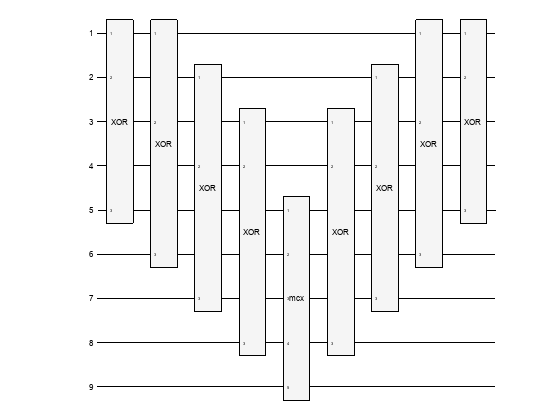
Plot the final circuit for the state oracle.

plot(oracle)

Check Final State Oracle Behavior

To check the behavior of the state oracle, use the same two input bit strings as before. Start with the invalid graph coloring 1111, where all nodes are the same color.

invalidColors = "11110000-";
inputState1 = quantum.gate.QuantumState(invalidColors);
formula(inputState1)

ans = 
"1 * |11110000->"

Apply the oracle to see the output state.

outputState1 = simulate(oracle,inputState1); 
formula(outputState1)

ans = 
"1 * |11110000->"

The oracle correctly determines that the graph coloring is not valid. The phase of the output bits is unchanged. Next, check the coloring 1001.

validColors = "10010000-";
inputState2 = quantum.gate.QuantumState(validColors);
formula(inputState2)

ans = 
"1 * |10010000->"

Again, apply the oracle to see the output state.

outputState2 = simulate(oracle,inputState2);
formula(outputState2)

ans = 
"(-1-3.8858e-16i) * |10010000->"

In this case, the state oracle correctly flips the phase to -1 because the graph coloring is valid. The small nonzero imaginary part is due to floating-point round-off error.

State Oracle Code

This function creates a state oracle circuit for a specified input graph.

function oracle = oracleGraphColoring(g)

xorInnerGates = [cxGate(1,3);
                 cxGate(2,3)];
xorGate = quantumCircuit(xorInnerGates,Name="XOR");

[startNodes,endNodes] = findedge(g);
N = numnodes(g);
E = numedges(g);

gates = [];
for k = 1:E
  gates = [gates; 
           compositeGate(xorGate,[startNodes(k),endNodes(k),N+k])];
end

lastQubit = N+E+1;
gates = [gates; mcxGate(N+(1:E),lastQubit,[])];
oracle = quantumCircuit(gates,lastQubit);
oracle.Name = "Oracle";

oracle.Gates = [oracle.Gates; 
                flip(oracle.Gates(1:end-1))];

end

Create Diffuser Circuit

Grover's algorithm combines a state oracle with a diffuser. The combined action of these two composite gates is a reflection in the plane spanned by $\left|\mathit{e}\right.anglebracketright$ (a vector of all equal values representing a superposition of all states) and $\left|\mathit{t}\right.anglebracketright$ (the target state). The diffuser applies the reflection ${\mathit{I}}_{\mathit{N}}-2\left|\mathit{e}\right.anglebracketright\left.anglebracketleft\mathit{e}\right|$.

Diffuser Code

This function creates a diffuser circuit with a specified number of nodes. Save this function in a file on the MATLAB path.

function cg = diffuser(n)
gates = [hGate(1:n);
         xGate(1:n);
         hGate(n);
         mcxGate(1:n-1, n, []);
         hGate(n);
         xGate(1:n);
         hGate(1:n)];
cg = quantumCircuit(gates,Name="Diffuser");
end

Check Diffuser Behavior

Create a diffuser circuit for the four-node graph coloring problem and plot the circuit.

diffuserG = diffuser(N);
plot(diffuserG)

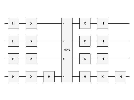
Verify that the diffuser applies a reflection of ${\mathit{I}}_{\mathit{N}}-2\left|\mathit{e}\right.anglebracketright\left.anglebracketleft\mathit{e}\right|$ by comparing the circuit matrix of diffuserG with a manually constructed reflection matrix.

e = ones(2^N,1);
e = e/norm(e);
M = eye(2^N) - 2*(e*e');
norm(getMatrix(diffuserG) - M)

ans = 1.0270e-15

The result is zero (up to round-off error), which confirms that the diffuser circuit applies the expected reflection.

Apply Grover's Algorithm to Graph Coloring Oracle

First, create a quantum circuit with the number of qubits required by the oracle. Bring the qubits representing node colors into superposition by applying hGate. Bringing these qubits into superposition represents all combinations of states equally, which is a common step at the beginning of quantum algorithms. Then, set the last qubit into state $\left|-\right.anglebracketright$ by applying xGate followed by hGate.

gates = [hGate(1:N);
         xGate(oracle.NumQubits);
         hGate(oracle.NumQubits)];
c = quantumCircuit(gates);

Check the circuit setup to make sure it produces the expected state.

s = simulate(c);
formula(s)

ans = 
"1 * |++++0000->"

Express the formula in the Z basis to confirm that all combinations of states are represented equally.

formula(s, Basis="Z")

ans = 
    "0.17678  * |000000000> +
     -0.17678 * |000000001> +
     0.17678  * |000100000> +
     -0.17678 * |000100001> +
     0.17678  * |001000000> +
     -0.17678 * |001000001> +
     0.17678  * |001100000> +
     -0.17678 * |001100001> +
     0.17678  * |010000000> +
     -0.17678 * |010000001> +
     0.17678  * |010100000> +
     -0.17678 * |010100001> +
     0.17678  * |011000000> +
     -0.17678 * |011000001> +
     0.17678  * |011100000> +
     -0.17678 * |011100001> +
     0.17678  * |100000000> +
     -0.17678 * |100000001> +
     0.17678  * |100100000> +
     -0.17678 * |100100001> +
     0.17678  * |101000000> +
     -0.17678 * |101000001> +
     0.17678  * |101100000> +
     -0.17678 * |101100001> +
     0.17678  * |110000000> +
     -0.17678 * |110000001> +
     0.17678  * |110100000> +
     -0.17678 * |110100001> +
     0.17678  * |111000000> +
     -0.17678 * |111000001> +
     0.17678  * |111100000> +
     -0.17678 * |111100001>"

Next, apply the oracle and diffuser composite gates two times in the circuit and then plot the resulting circuit. (The number of times that the oracle and diffuser need to be applied depends on the angle of rotation for a given problem, which can be determined based on what percentage of the possible inputs are valid. You can try applying the oracle and diffuser different numbers of times to view the effect on the outputs.)

gates = [gates;
         compositeGate(oracle,1:9);
         compositeGate(diffuserG,1:4);
         compositeGate(oracle,1:9);
         compositeGate(diffuserG,1:4)];
c = quantumCircuit(gates);
plot(c)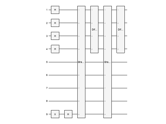

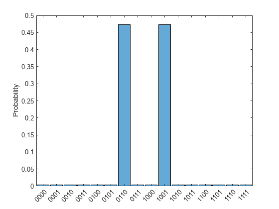
Simulate the circuit to see which node colorings are most likely to be measured. Plot a histogram of the results for the first four qubits.

s = simulate(c);
histogram(s,1:4)

Use querystates to view the same information as a table.

[outputBits,probabilities] = querystates(s,1:4);
T = table(outputBits,probabilities);
T = sortrows(T,"probabilities","descend")

T=16×2 table
    outputBits    probabilities
    __________    _____________

      "0110"          0.47266  
      "1001"          0.47266  
      "0100"        0.0039063  
      "1011"        0.0039063  
      "0011"        0.0039063  
      "1100"        0.0039063  
      "0001"        0.0039063  
      "0010"        0.0039063  
      "0101"        0.0039063  
      "1010"        0.0039063  
      "1101"        0.0039063  
      "1110"        0.0039063  
      "0111"        0.0039063  
      "1000"        0.0039063  
      "0000"        0.0039062  
      "1111"        0.0039062  

The simulation results show that the two states most likely to be measured are 0110 and 1001, which are the two possible valid graph colorings.

Run Circuit on AWS®

Simulating a circuit locally can give an indication of the most probable results on a quantum machine, but running actual calculations on a quantum machine still has probabilistic results. Therefore, it is common to run the same circuit several times on a quantum machine to get a good estimate of the probability of each output. The number of trials is referred to as the number of shots.

To run circuits on AWS®, you need an AWS® account with access to AWS® Braket. See Run Quantum Circuit on Hardware Using AWS for more information on how to set up access and see available devices.

First, connect to a quantum device using quantum.backend.QuantumDeviceAWS. Specify the name of the device as well as its region and the path of the bucket to store results.

reg = "us-east-1";
bucketPath = "s3://amazon-braket-mathworks/doc-examples";
device = quantum.backend.QuantumDeviceAWS("SV1",Region=reg,S3Path=bucketPath)

device = 
  QuantumDeviceAWS with properties:

         Name: "SV1"
    DeviceARN: "arn:aws:braket:::device/quantum-simulator/amazon/sv1"
       Region: "us-east-1"
       S3Path: "s3://amazon-braket-mathworks/doc-examples"

Create a task to run the circuit on the device. By default, run uses 100 shots.

task = run(c,device)

task = 
  QuantumTaskAWS with properties:

    TaskARN: "arn:aws:braket:us-east-1:532578954166:quantum-task/342f9043-39ec-493e-a12b-4ba57b043a78"
     Status: "finished"

Quantum devices have limited availability, so tasks are often queued for execution. Once the task is finished, the Status property of the task object has a value of "finished". Check the status of the task by querying the Status property periodically, or use the wait method to internally check the status until the task is finished.

if ~strcmp(task.Status,"finished")
    wait(task)
end

Once the task is finished, retrieve the result of running the circuit by using fetchOutput.

R = fetchOutput(task)

R = 
  QuantumMeasurement with properties:

    MeasuredStates: [8×1 string]
            Counts: [8×1 double]
     Probabilities: [8×1 double]
         NumQubits: 9

Display the measurement results for the circuit.

T = table(R.Counts,R.Probabilities,R.MeasuredStates, ...
    VariableNames=["Counts","Probabilities","States"])

T=8×3 table
    Counts    Probabilities      States   
    ______    _____________    ___________

       1          0.01         "010000000"
       1          0.01         "010100001"
      29          0.29         "011000000"
      19          0.19         "011000001"
       1          0.01         "011100000"
      16          0.16         "100100000"
      32          0.32         "100100001"
       1          0.01         "110000001"

Plot a histogram of the results for the first four qubits, which correspond to the node colors.

histogram(R,1:4)

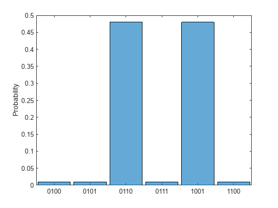
The results agree with the local simulation, showing 0110 and 1001 as valid graph colorings. The results solve the graph coloring problem by indicating that nodes 2 and 3 in the graph can be the same color and that nodes 1 and 4 can be the same color.