Solve ODE with Strongly State-Dependent Mass Matrix
This example shows how to solve Burgers' equation using a moving mesh technique [1]. The problem includes a mass matrix, and options are specified to account for the strong state dependence and sparsity of the mass matrix, making the solution process more efficient.
Problem Setup
Burgers' equation is a convection-diffusion equation given by the PDE
Applying a coordinate transformation (Eq. 18 in [1]) leads to an extra term on the left-hand side:
Converting the PDE into an ODE of one variable is accomplished by using finite differences to approximate the partial derivatives taken with respect to . If the finite differences are written as , then the PDE can be rewritten as an ODE that only contains derivatives taken with respect to :
In this form, you can use an ODE solver such as ode15s to solve for and over time.
For this example, the problem is formulated on a moving mesh of points, and the moving mesh technique described in [1] positions the mesh points at each time step so that they are concentrated in areas of change. The boundary and initial conditions are
For a given initial mesh of points, there are equations to solve: equations corresponding to Burgers' equation, and equations determining the movement of each mesh point. So, the final system of equations is:
The terms for the moving mesh correspond to MMPDE6 in [1]. The parameter represents a timescale for forcing the mesh toward equidistribution. The term is a monitor function given by Eq. 21 in [1]:
The approach used in this example to solve Burgers' equation with moving mesh points demonstrates several techniques:
The system of equations is expressed using a mass matrix formulation, . The mass matrix is provided to the
ode15ssolver as a function.The derivative function not only includes the equations for Burgers' equation, but also a set of equations governing the moving mesh selection.
The sparsity patterns of the Jacobian and the derivative of the mass matrix multiplied with a vector are supplied to the solver as functions. Supplying these sparsity patterns helps the solver operate more efficiently.
Finite differences are used to approximate several partial derivatives.
To solve this equation in MATLAB®, write a derivative function, a mass matrix function, a function for the sparsity pattern of the Jacobian , and a function for the sparsity pattern of . You can either include the required functions as local functions at the end of a file (as done here), or save them as separate, named files in a directory on the MATLAB path.
Code Mass Matrix
The left side of the system of equations involves linear combinations of first derivatives, so a mass matrix is required to represent all of the terms. Set the left side of the system of equations equal to to extract the form of the mass matrix. The mass matrix is composed of four blocks, each of which is a square matrix of order :
.
This formulation shows that and form the left side of Burgers' equations (the first equations in the system), while and form the left side of the mesh equations (the last equations in the system). The block matrices are:
is the identity matrix. The partial derivatives in are estimated using finite differences, while the partial derivative in uses a Laplacian matrix. Notice that contains only zeros because none of the equations for the mesh movement depend on .
Now you can write a function that computes the mass matrix. The function must accept two inputs for time and the solution vector . Since the solution vector contains half components and half components, the function extracts these first. Then, the function forms all of the block matrices (taking the boundary values of the problem into account) and assembles the mass matrix using the four blocks.
function M = mass(t,y)
% Extract the components of y for the solution u and mesh x
N = length(y)/2;
u = y(1:N);
x = y(N+1:end);

% Boundary values of solution u and mesh x
u0 = 0;
uNP1 = 0;
x0 = 0;
xNP1 = 1;

% M1 and M2 are the portions of the mass matrix for Burgers' equation.
% The derivative du/dx is approximated with finite differences, using
% single-sided differences on the edges and centered differences in between.
M1 = speye(N);
i = 2:N-1;
v = [0; -(u(i+1) - u(i-1))./(x(i+1) - x(i-1)) ; 0];
M2 = spdiags(v,0,N,N);

M2(1,1) = - (u(2) - u0)/(x(2) - x0);
M2(N,N) = - (uNP1 - u(N-1))/(xNP1 - x(N-1));

% M3 and M4 define the equations for mesh point evolution, corresponding to
% MMPDE6 in the reference paper. Since the mesh functions only involve d/dt(dx/dt),
% the M3 portion of the mass matrix is all zeros. The second derivative in M4 is
% approximated using a finite difference Laplacian matrix.
M3 = sparse(N,N);
M4 = spdiags([1 -2 1],-1:1,N,N);

% Assemble mass matrix
M = [M1 M2; M3 M4];
end
Note: All functions are included as local functions at the end of the example.
Code Derivative Function
The derivative function for this problem returns a vector with elements. The first elements correspond to Burgers' equations, while the last elements are for the moving mesh equations. The function movingMeshODE goes through these steps to evaluate the right-hand sides of all the equations in the system:
Evaluate Burgers' equations using finite differences (first elements).
Evaluate monitor function (last elements).
Apply spatial smoothing to monitor function and evaluate moving mesh equations.
The first equations in the derivative function encode the right side of Burgers' equations. Burgers' equations can be considered as a differential operator involving spatial derivatives of the form:
.
The reference paper [1] describes the process of approximating the differential operator using centered finite differences by
On the edges of the mesh (for which and ), only single-sided differences are used instead. This example uses .
The equations governing the mesh (comprising the last equations in the derivative function) are
Just as with Burgers' equations, you can use finite differences to approximate the monitor function :
Once the monitor function is evaluated, spatial smoothing is applied (Equations 14 and 15 in [1]). This example uses and for the spatial smoothing parameters.
The function encoding the system of equations is
function g = movingMeshODE(t,y)
% Extract the components of y for the solution u and mesh x
N = length(y)/2;
u = y(1:N);
x = y(N+1:end);

% Boundary values of solution u and mesh x
u0 = 0;
uNP1 = 0;
x0 = 0;
xNP1 = 1;

% Preallocate g vector of derivative values.
g = zeros(2*N,1);

% Use centered finite differences to approximate the RHS of Burgers'
% equations (with single-sided differences on the edges). The first N
% elements in g correspond to Burgers' equations.
ind = 1:N;
x = [x0; x; xNP1];
u = [u0; u; uNP1];
i = 2:N+1;
delx = x(i+1) - x(i-1);
g(ind) = 1e-4*((u(i+1) - u(i))./(x(i+1) - x(i)) - ...
          (u(i) - u(i-1))./(x(i) - x(i-1)))./(0.5*delx) - ...
          0.5*(u(i+1).^2 - u(i-1).^2)./delx;

% Evaluate the monitor function values (Eq. 21 in reference paper), used in
% RHS of mesh equations. Centered finite differences are used for interior
% points, and single-sided differences are used on the edges.
M = zeros(N,1);
M(ind) = sqrt(1 + ((u(i+1) - u(i-1))./(x(i+1) - x(i-1))).^2);
M0 = sqrt(1 + ((u(2) - u0)/(x(2) - x0))^2);
MNP1 = sqrt(1 + ((uNP1 - u(N+1))/(xNP1 - x(N+1)))^2);

% Apply spatial smoothing (Eqns. 14 and 15) with gamma = 2, p = 2.
x = y(N+1:end);
ind = 2:N-1;
SM = zeros(N,1);
i = 3:N-2;
SM(i) = sqrt((4*M(i-2).^2 + 6*M(i-1).^2 + 9*M(i).^2 + ...
    6*M(i+1).^2 + 4*M(i+2).^2)/29);

SM0 = sqrt((9*M0^2 + 6*M(1)^2 + 4*M(2)^2)/19);
SM(1) = sqrt((6*M0^2 + 9*M(1)^2 + 6*M(2)^2 + 4*M(3)^2)/25);
SM(2) = sqrt((4*M0^2 + 6*M(1)^2 + 9*M(2)^2 + 6*M(3)^2 + 4*M(4)^2)/29);
SM(N-1) = sqrt((4*M(N-3)^2 + 6*M(N-2)^2 + 9*M(N-1)^2 + 6*M(N)^2 + 4*MNP1^2)/29);
SM(N) = sqrt((4*M(N-2)^2 + 6*M(N-1)^2 + 9*M(N)^2 + 6*MNP1^2)/25);
SMNP1 = sqrt((4*M(N-1)^2 + 6*M(N)^2 + 9*MNP1^2)/19);

g(ind+N) = (SM(ind+1) + SM(ind)).*(x(ind+1) - x(ind)) - ...
    (SM(ind) + SM(ind-1)).*(x(ind) - x(ind-1));
g(1+N) = (SM(2) + SM(1))*(x(2) - x(1)) - (SM(1) + SM0)*(x(1) - x0);
g(N+N) = (SMNP1 + SM(N))*(xNP1 - x(N)) - (SM(N) + SM(N-1))*(x(N) - x(N-1));

% Form final discrete approximation for Eq. 12 in reference paper, the equation governing
% the mesh points.
tau = 1e-3;
g(1+N:end) = - g(1+N:end)/(2*tau);
end
Code Functions for Sparsity Patterns
The Jacobian for the derivative function is a matrix containing all of the partial derivatives of the derivative function, movingMeshODE. ode15s estimates the Jacobian using finite differences when the matrix is not supplied in the options structure. You can supply the sparsity pattern of the Jacobian to help ode15s calculate it more quickly.
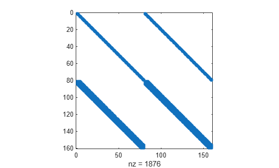
The function for the sparsity pattern of the Jacobian is
function out = JPat(N)
S1 = spdiags(1,-1:1,N,N);
S2 = spdiags(1,-4:4,N,N);
out = [S1 S1; S2 S2];
end
Plot the sparsity pattern of for using spy.
spy(JPat(80))
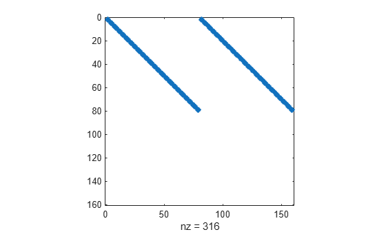
Another way to make the calculation more efficient is to provide the sparsity pattern of . You can find this sparsity pattern by examining which terms of and are present in the finite differences calculated in the mass matrix function.
The function for the sparsity pattern of is
function S = MvPat(N)
SZ = sparse(N,N);
S1 = spdiags(1,[-1 1],N,N);
S = [S1 S1; SZ SZ];
end
Plot the sparsity pattern of for using spy.
spy(MvPat(80))
Solve System of Equations
Solve the system with the value . For the initial conditions, initialize with a uniform grid and evaluate on the grid.
N = 80;
h = 1/(N+1);
xinit = h*(1:N);
uinit = sin(2*pi*xinit) + 0.5*sin(pi*xinit);
y0 = [uinit xinit];
Use odeset to create an options structure that sets several values:
A function handle for the mass matrix
The state-dependence of the mass matrix, which for this problem is
'strong'since the mass matrix is a function of both andA function handle that calculates the Jacobian sparsity pattern
A function handle that calculates the sparsity pattern of the derivative of the mass matrix multiplied by a vector
The absolute and relative error tolerances
opts = odeset(Mass=@mass,MStateDependence="strong",JPattern=JPat(N),...
       MvPattern=MvPat(N),RelTol=1e-5,AbsTol=1e-4);
Finally, call ode15s to solve the system on the interval using the movingMeshODE derivative function, the time span, the initial conditions, and the options structure.
tspan = [0 1];
sol = ode15s(@movingMeshODE,tspan,y0,opts);
Plot Results
The result of the integration is a structure sol that contains the time steps , the mesh points , and the solution . Extract these values from the structure.
t = sol.x;
x = sol.y(N+1:end,:);
u = sol.y(1:N,:);
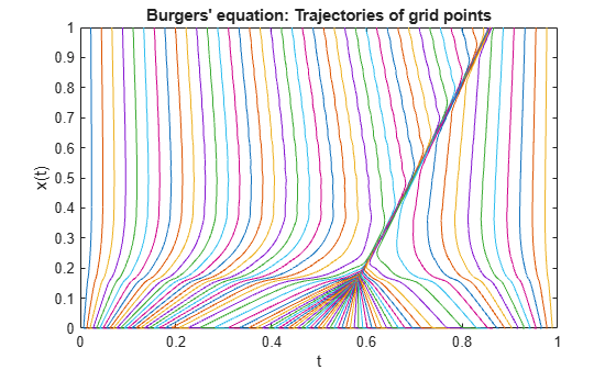
Plot the movement of the mesh points over time. The plot shows that the mesh points retain a reasonably even spacing over time (due to the monitor function), but they are able to cluster near the discontinuity in the solution as it moves.
plot(x,t)
xlabel("t")
ylabel("x(t)")
title("Burgers' equation: Trajectories of grid points")
Now, sample at a few values of and plot the evolution of the solution over time. The mesh points at the ends of the interval are fixed, so x(0) = 0 and x(N+1) = 1. The boundary values are u(t,0) = 0 and u(t,1) = 0, which you must add to the known values computed for the figure.
tint = 0:0.2:1;
yint = deval(sol,tint);
figure
labels = {};
for j = 1:length(tint)
   solution = [0; yint(1:N,j); 0];
   location = [0; yint(N+1:end,j); 1];
   labels{j} = ['t = ' num2str(tint(j))];
   plot(location,solution,"-o")
   hold on
end
xlabel("x")
ylabel("solution u(x,t)")
legend(labels{:},"Location","SouthWest")
title("Burgers equation on moving mesh")
hold off
The plot shows that is a smooth wave that develops a steep gradient over time as it moves towards . The mesh points track the movement of the discontinuity so that extra evaluation points are in the appropriate position in each time step.
References
[1] Huang, Weizhang, et al. “Moving Mesh Methods Based on Moving Mesh Partial Differential Equations.” Journal of Computational Physics, vol. 113, no. 2, Aug. 1994, pp. 279–90. https://doi.org/10.1006/jcph.1994.1135.
Local Functions
Listed here are the local helper functions that the solver ode15s calls to calculate the solution. Alternatively, you can save these functions as their own files in a directory on the MATLAB path.
function g = movingMeshODE(t,y)
% Extract the components of y for the solution u and mesh x
N = length(y)/2;
u = y(1:N);
x = y(N+1:end);

% Boundary values of solution u and mesh x
u0 = 0;
uNP1 = 0;
x0 = 0;
xNP1 = 1;

% Preallocate g vector of derivative values.
g = zeros(2*N,1);

% Use centered finite differences to approximate the RHS of Burgers'
% equations (with single-sided differences on the edges). The first N
% elements in g correspond to Burgers' equations.
ind = 1:N;
x = [x0; x; xNP1];
u = [u0; u; uNP1];
i = 2:N+1;
delx = x(i+1) - x(i-1);
g(ind) = 1e-4*((u(i+1) - u(i))./(x(i+1) - x(i)) - ...
          (u(i) - u(i-1))./(x(i) - x(i-1)))./(0.5*delx) - ...
          0.5*(u(i+1).^2 - u(i-1).^2)./delx;

% Evaluate the monitor function values (Eq. 21 in reference paper), used in
% RHS of mesh equations. Centered finite differences are used for interior
% points, and single-sided differences are used on the edges.
M = zeros(N,1);
M(ind) = sqrt(1 + ((u(i+1) - u(i-1))./(x(i+1) - x(i-1))).^2);
M0 = sqrt(1 + ((u(2) - u0)/(x(2) - x0))^2);
MNP1 = sqrt(1 + ((uNP1 - u(N+1))/(xNP1 - x(N+1)))^2);

% Apply spatial smoothing (Eqns. 14 and 15) with gamma = 2, p = 2.
x = y(N+1:end);
ind = 2:N-1;
SM = zeros(N,1);
i = 3:N-2;
SM(i) = sqrt((4*M(i-2).^2 + 6*M(i-1).^2 + 9*M(i).^2 + ...
    6*M(i+1).^2 + 4*M(i+2).^2)/29);

SM0 = sqrt((9*M0^2 + 6*M(1)^2 + 4*M(2)^2)/19);
SM(1) = sqrt((6*M0^2 + 9*M(1)^2 + 6*M(2)^2 + 4*M(3)^2)/25);
SM(2) = sqrt((4*M0^2 + 6*M(1)^2 + 9*M(2)^2 + 6*M(3)^2 + 4*M(4)^2)/29);
SM(N-1) = sqrt((4*M(N-3)^2 + 6*M(N-2)^2 + 9*M(N-1)^2 + 6*M(N)^2 + 4*MNP1^2)/29);
SM(N) = sqrt((4*M(N-2)^2 + 6*M(N-1)^2 + 9*M(N)^2 + 6*MNP1^2)/25);
SMNP1 = sqrt((4*M(N-1)^2 + 6*M(N)^2 + 9*MNP1^2)/19);

g(ind+N) = (SM(ind+1) + SM(ind)).*(x(ind+1) - x(ind)) - ...
    (SM(ind) + SM(ind-1)).*(x(ind) - x(ind-1));
g(1+N) = (SM(2) + SM(1))*(x(2) - x(1)) - (SM(1) + SM0)*(x(1) - x0);
g(N+N) = (SMNP1 + SM(N))*(xNP1 - x(N)) - (SM(N) + SM(N-1))*(x(N) - x(N-1));

% Form final discrete approximation for Eq. 12 in reference paper, the equation governing
% the mesh points.
tau = 1e-3;
g(1+N:end) = - g(1+N:end)/(2*tau);
end

% -----------------------------------------------------------------------
function M = mass(t,y)
% Extract the components of y for the solution u and mesh x
N = length(y)/2;
u = y(1:N);
x = y(N+1:end);

% Boundary values of solution u and mesh x
u0 = 0;
uNP1 = 0;
x0 = 0;
xNP1 = 1;

% M1 and M2 are the portions of the mass matrix for Burgers' equation.
% The derivative du/dx is approximated with finite differences, using
% single-sided differences on the edges and centered differences in between.
M1 = speye(N);
i = 2:N-1;
v = [0; -(u(i+1) - u(i-1))./(x(i+1) - x(i-1)) ; 0];
M2 = spdiags(v,0,N,N);

M2(1,1) = - (u(2) - u0)/(x(2) - x0);
M2(N,N) = - (uNP1 - u(N-1))/(xNP1 - x(N-1));

% M3 and M4 define the equations for mesh point evolution, corresponding to
% MMPDE6 in the reference paper. Since the mesh functions only involve d/dt(dx/dt),
% the M3 portion of the mass matrix is all zeros. The second derivative in M4 is
% approximated using a finite difference Laplacian matrix.
M3 = sparse(N,N);
M4 = spdiags([1 -2 1],-1:1,N,N);

% Assemble mass matrix
M = [M1 M2; M3 M4];
end

% -------------------------------------------------------------------------
function out = JPat(N)  % Jacobian sparsity pattern
S1 = spdiags(1,-1:1,N,N);
S2 = spdiags(1,-4:4,N,N);
out = [S1 S1; S2 S2];
end

% -------------------------------------------------------------------------
function S = MvPat(N)  % Sparsity pattern for the derivative of the Mass matrix times a vector
SZ = sparse(N,N);
S1 = spdiags(1,[-1 1],N,N);
S = [S1 S1; SZ SZ];
end
% -------------------------------------------------------------------------