Estimate Battery State of Charge Using Deep Learning with ESP32 Board
This example shows how to estimate the state of charge (SOC) of a battery using a deep learning model in MATLAB® with an ESP32-based hardware setup.
SOC represents the remaining charge of an electric battery as a percentage of its total capacity. This example uses experimentally characterized data collected from a battery at five different ambient temperatures. The obtained data set has three input features, current, voltage, and temperature, and one output feature, SOC. In this example, you prepare this data set to train and test a long short-term memory (LSTM) neural network that predicts SOC based on the three input features.
This example uses an ESP32-based development kit connected to MATLAB as a demonstration setup for real-time SOC prediction. In this setup, the battery powers a DC geared motor that acts as a variable load, while sensors monitor the electrical and thermal behavior of the battery. You use MATLAB to communicate with the ESP32 development kit, read sensor data in real time, apply the trained deep learning model to estimate the SOC, and send the predicted value back to the ESP32 for display on its on-board LCD.
Note: ESP32 hardware is not supported in MATLAB® Online™. Use the installed version of MATLAB to run this example.
Required Hardware
M5Stack Core2 ESP32 IoT Development Kit — ESP32-based microcontroller with Arduino support
CJMCU-219 INA219 — Bidirectional current sensor
LM35 — Temperature sensor
BAK N18650 — Lithium-ion battery
1.8V – 12V/2A PWM Speed Regulator — DC-motor speed controller
300 RPM BO Motor-Straight — DC geared motor
Prepare Data for Battery State of Charge (SOC) Estimation
In practice, the battery data is collected at various ambient temperatures by experimental characterization. For more information, see Characterize Battery Cell for Electric Vehicles (Simscape Battery). For this example, load the provided battery data instead. This data consists of five MAT files, each corresponding to a different ambient temperature: 0, 10, 25, 35 and 45 degrees Celsius.
% Set the random number generator to default for reproducibility
rng("default")

load(fullfile("batteryData","testData0degC.mat"));
load(fullfile("batteryData","testData10degC.mat"));
load(fullfile("batteryData","testData25degC.mat"));
load(fullfile("batteryData","testData35degC.mat"));
load(fullfile("batteryData","testData45degC.mat"));
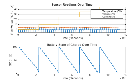
Each data set represents a specific temperature condition and is stored in a structure with fields X and Y. The field X is an array containing sensor readings, including current, voltage, and temperature. The field Y is an array containing the corresponding state-of-charge (SoC) values. To create a unified data set across all temperature conditions, concatenate the X arrays from each structure into a single variable X, and the Y arrays into a single variable Y.
X = [testData0degC.X; testData10degC.X; testData25degC.X; testData35degC.X; testData45degC.X];
Y = [testData0degC.Y; testData10degC.Y; testData25degC.Y; testData35degC.Y; testData45degC.Y];
Visualize the combined data.
figure
tiledlayout(2,1)

nexttile
plot(X)
legend(["Temperature (°C)","Voltage (V)","Current (A)"])
xlabel("Time (Seconds)")
ylabel("Raw Value (°C / V / A)")
title("Sensor Readings Over Time")
grid on

nexttile
plot(Y*100,'LineWidth',1.5)
xlabel("Time (Seconds)")
ylabel("SOC (%)")
title("Battery State of Charge Over Time")
grid on
Prepare the data for training an LSTM deep learning model by splitting the data into chunks of 500 samples. First, calculate the number of resulting data chunks.
chunkSize = 500;

numSamples = length(Y);
numObservations = floor(numSamples / chunkSize);
Preallocate cell arrays to hold the chunked data. Then, loop over the number of data chunks to populate the cell arrays. Discard any remaining data.
XData = cell(1, numObservations);
YData = cell(1, numObservations);

for i = 1:numObservations
    idxStart = 1 + (i - 1) * chunkSize;
    idxEnd = i * chunkSize;
    XData{i} = X(idxStart:idxEnd, :);
    YData{i} = Y(idxStart:idxEnd);
end
To create a model that is representative and unbiased, randomly shuffle the indices of all observations before splitting them into training and validation sets. Use 70% of the data for training and 30% for validation.
idx = randperm(numObservations);
numObservationsTrain = floor(0.7 * numObservations);
idxTrain = idx(1:numObservationsTrain);
numObservationsValidation = numObservations - numObservationsTrain;
idxValidation = idx(numObservationsTrain + 1:end);

XTrain = XData(idxTrain);
YTrain = YData(idxTrain);
XVal = XData(idxValidation);
YVal = YData(idxValidation);
Visualize one training observation.
idx = 1;
figure
tiledlayout(2,1)

nexttile
plot(XTrain{idx},'LineWidth',1.2)
legend(["Temperature (°C)","Voltage (V)","Current (A)"])
xlabel("Time (Seconds)")
ylabel("Raw Value (°C / V / A)")
title("Sensor Measurements Over Time")
grid on

nexttile
plot(YTrain{idx}*100,'LineWidth',1.5,'Color',[0.1 0.5 0.8])
xlabel("Time (Seconds)")
ylabel("SOC (%)")
title("Battery State of Charge Over Time")
grid on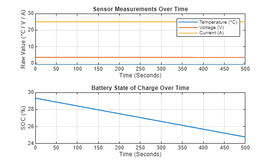
Train and Test Prediction Model
The network architecture and training settings in this section are optimized for the use case shown in this example. For guidance on customizing deep learning models and training strategies, see Train Deep Learning Network for Battery State of Charge Estimation (Deep Learning Toolbox).
Set the number of input and output features for your training network. In this example, current, voltage, and temperature are input features, and SOC is the output feature.
numFeatures = 3;
numResponses = 1;
Define the LSTM network architecture with two LSTM layers and two dropout layers.
layers = [...
    sequenceInputLayer(numFeatures)
    lstmLayer(256,OutputMode="sequence")
    dropoutLayer(0.2)
    lstmLayer(128,OutputMode="sequence")
    dropoutLayer(0.2)
    fullyConnectedLayer(numResponses)
    sigmoidLayer];
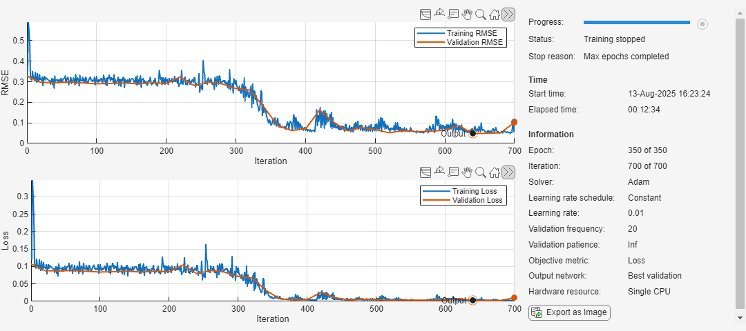
Set the training options for the deep learning network using the trainingOptions (Deep Learning Toolbox) function. This example uses the Adam optimizer with a 0.01 learning rate, trains for 350 epochs with a mini-batch size of 64, and left-pads sequences to standardize lengths. The example also shuffles data each epoch, monitors RMSE every 20 iterations, visualizes progress with plots, and disables verbose output.
options = trainingOptions("adam", ...
    InitialLearnRate=0.01, ...
    MaxEpochs=350, ...
    MiniBatchSize=64, ...
    SequencePaddingDirection="left", ...
    Shuffle="every-epoch",...
    ValidationData={XVal,YVal}, ...
    ValidationFrequency=20, ...
    Plots="training-progress", ...
    Metrics="rmse", ...
    Verbose=false);
To train the LSTM network using the trainnet (Deep Learning Toolbox) function, set the doTraining flag to true. When doTraining is false, the example loads a pretrained network that was trained using the data and training parameters defined previously.
doTraining = false;

if doTraining
    recurrentNet = trainnet(XTrain,YTrain,layers,"mse",options);
else
    load("pretrainedBSOCNetwork.mat");
end
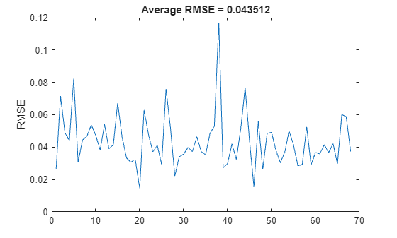
To test the prediction model, use the trained LSTM network to predict the SOC on the validation data. Then, compute the root mean squared error (RMSE) between the predicted and target SOC values for each validation set.
YPred = minibatchpredict(recurrentNet,XVal);
TestRMSE = [];

for i = 1:length(XVal)
    residuals = YVal{1,i} - YPred(:,:,i);
    TestRMSE = [TestRMSE; sqrt(mean(residuals.^2))];
end
Visualize the RMSE for each validation sequence. A lower RMSE indicates higher prediction accuracy. The LSTM network used in this example has an average RMSE of about 0.0435.
figure
plot(TestRMSE)
ylabel("RMSE")
title("Average RMSE = " + num2str(mean(TestRMSE)))
Hardware Setup
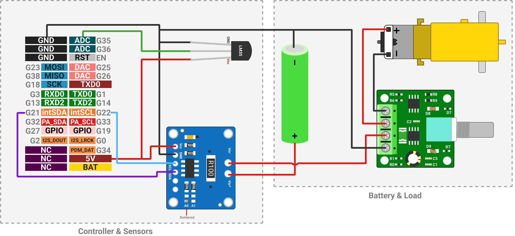
Now that you have trained and tested the predictive model, you can build a hardware setup for SOC prediction by completing these circuit connections.
Connect the M5Stack Core2 to the computer via USB and configure it in the Hardware Setup window by selecting
ESP32-WROOM-DevKitV1. For more information, see Set Up and Configure Arduino Hardware.Connect the DC geared motor to the speed controller.
To interface the INA219 sensor with the I2C address
0x41, solder theA0pin of the sensor.Connect the
SDAandSCLpins of the INA219 sensor to theintSDAandintSCLpins on the M5Stack Core2.Connect the
Outpin of the temperature sensor to theA0pin of the Arduino on the M5Stack Core2.Connect the
Vccpins of all sensors to the5Vpin on the M5Stack Core2.Connect the positive terminal of the battery to the
Vin+pin of the current sensor.Connect the
Vin-pin of the current sensor toPower+pin of the speed controller.Establish a common ground between the battery-powered load circuit and the sensors powered by the M5Stack Core2. To do so, connect the negative terminal of the battery, along with the
GNDpins of the temperature sensor, current sensor, and speed controller, to aGNDpin on the M5Stack Core2.
Integrate ESP32 Sensor Interface with MATLAB Prediction Model
To estimate the SOC of a battery in real time, integrate the prediction model with the hardware system. To interface with the INA219 sensor and M5Core2 on-board LCD, you need the custom Arduino Add-On libraries provided with this example, Adafruit INA219 and M5Core2. Check for these libraries, and if needed, install them using the helper functions also provided.
if ~arduinoio.isLibraryInstalled('Adafruit INA219')
    arduinoio.CLIInstallLibrary('Adafruit INA219');
end
if ~arduinoio.isLibraryInstalled('M5Core2')
    arduinoio.CLIInstallLibrary('M5Core2');
end
Create an Arduino object with Adafruit INA219 and M5Core2 LCD libraries using the arduino function. This example uses an ESP32-WROOM-DevKitV1 connected via COM port 8 to the host computer. You can update the COM port number based on the port information of your hardware board. For more information, see Find Arduino Port on Windows, Mac, and Linux.
aObj = arduino("COM8","ESP32-WROOM-DevKitV1","Libraries",{"ExampleAddon/MyINA219","ExampleAddon/MyM5LCD","I2C"});
Create add-on objects for the INA219 sensor and M5Stack Core2 on-board LCD using the addon function. For the sensor, use I2C address 0x41, which is configured by soldering the A0 pin on the sensor as specified in the previous section.
sensor = addon(aObj,"ExampleAddon/MyINA219","I2CAddress",0x41);
lcd = addon(aObj,"ExampleAddon/MyM5LCD");
To read sensor data and predict SOC, every second for a hundred seconds:
Read the current, voltage, and temperature from the sensor. Convert the current value obtained in mA from the INA219 sensor to A (Amperes). This example uses an LM35 temperature sensor with a sensitivity of 10 mV/°C, so multiply the voltage read from the sensor by 100 to convert it to temperature in °C.
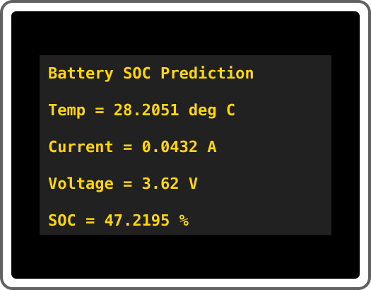
Use the trained LSTM network to predict the SOC and display the predicted value in the MATLAB command window.
Clear the on-board LCD screen of the M5Stack Core2 and print headings and sensor readings to the screen.
Wait for one second before the next reading.
for idx =1:100

    current = readCurrent(sensor)/1000;
    voltage = readVoltage(sensor);
    temperature = readVoltage(aObj,'D35')*100;

    out = predict(recurrentNet,[current,voltage,temperature]);
    disp(['SOC Status = ' num2str(out)]);

    clearLCD(lcd);
    printLCD(lcd, 'Battery SOC Prediction',0,0);
    printLCD(lcd, ['Temp = ' num2str(temperature) ' deg C'],0,30);
    printLCD(lcd, ['Current = ' num2str(current) ' A'],0,60);
    printLCD(lcd, ['Voltage = ' num2str(voltage) ' V'],0,90);
    printLCD(lcd, ['SOC = ' num2str(out*100) ' %'],0,120);

    pause(1);
end
Clean Up
When you no longer need the connections, clear the associated hardware objects.
clear aObj sensor lcd
See Also
Topics
- Battery State of Charge Estimation Using Deep Learning (Deep Learning Toolbox)